PSF Model Basics

Here we will cover some of the main ways to use PSF and point source models in AstroPhot. You will learn how to make a model with a PSF blurring kernel as well as define point sources in images.

%load_ext autoreload
%autoreload 2

import astrophot as ap
import numpy as np
import matplotlib.pyplot as plt

%matplotlib inline

PSF Images

A PSFImage is an AstroPhot object which stores the data for a point spread function (PSF). A PSF is fundamentally different from other image types, it only makes sense to describe a PSF in the pixel space of another image and so it has no WCS information to transform between pixel space, tangent plane, and world coordinates. It records the pixel values for the PSF as well as meta-data, mainly how upsampled the PSF is relative to the primary image. The point spread function is a description of how light is distributed into pixels when the light source is a delta function. In Astronomy we are blessed/cursed with many delta function like sources in our images and so PSF modelling is a major component of astronomical image analysis. Here are some points to keep in mind about a PSF.

• PSF images are always odd in shape (e.g. 25x25 pixels, not 24x24 pixels), at the center pixel, in the center of that pixel is where the delta function point source is located by definition

• The light in each pixel of a PSF image is already integrated. That is to say, the flux value for a pixel does not represent some model evaluated at the center of the pixel, it instead represents an integral over the whole area of the pixel

• PSF images can be assigned to a target image, or to individual models. If assigned to a target image all models acting on that target will use that PSF (unless they have their own which overrides it)

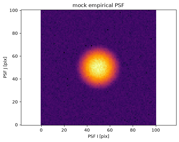
# An example fake "empirical PSF"
np.random.seed(124)
psf = ap.utils.initialize.gaussian_psf(2.0, 101, 0.5)
psf += 1e-7
psf += np.random.normal(scale=psf / 4)
psf[psf < 0] = ap.utils.initialize.gaussian_psf(2.0, 101, 0.5)[psf < 0]

psf_target = ap.PSFImage(data=psf, upsample=1)  # no upsampling

# To ensure the PSF has a normalized flux of 1, we call
psf_target.normalize()

fig, ax = plt.subplots()
ap.plots.psf_image(fig, ax, psf_target)
ax.set_title("mock empirical PSF")
plt.show()

# Dummy target for sampling purposes
target = ap.TargetImage(data=np.zeros((300, 300)), pixelscale=0.5, psf=psf_target)

Point Sources (star, super nova, distant galaxy, quasar, asteroid, etc.)

One of the most common astronomical sources is a point source. This is a source of light which is so small that it is, for all relevant purposes, infinitely small (a delta function). Though the point source may be extremely small, it’s footprint in an image is often quite extended, this is because the optics of a telescope, the intervening atmosphere, and a few other factors, work to broaden the light distribution that would otherwise fall entirely in a single pixel of the detector. The characterization of how the light is “blurred” is called a point spread function (PSF). In AstroPhot, there is one model "point model" which describes all point sources, this is a delta function which gets convolved by a PSF to produce an effect in an image. A point source is characterized by two measurements, the position (center), and the flux. Here we can see an example of how to set up a point source model.

pointsource = ap.Model(
    model_type="point model",
    target=target,
    center=[75.25, 75.9],
    flux=1,
    psf=psf_target,
)
pointsource.initialize()
# With a convolved sersic the center is much more smoothed out
fig, ax = plt.subplots(figsize=(6, 6))
ap.plots.model_image(fig, ax, pointsource, showcbar=False)
ax.set_title("Point source, with empirical PSF")
plt.show()

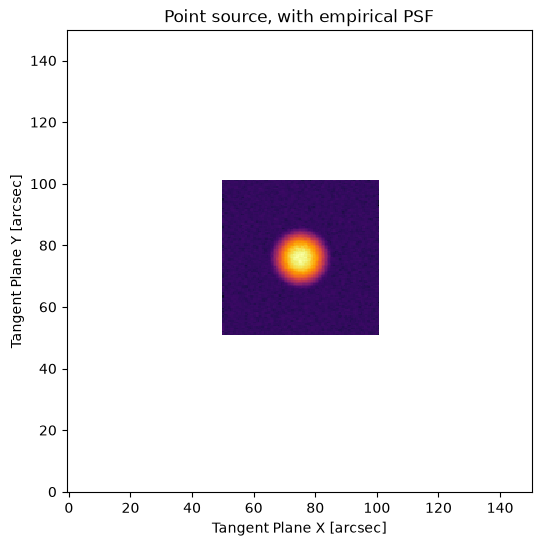
Don’t worry about the “fuzz” of values outside the PSF model. These values are of order 1e-18 and are an artefact of the sub-pixel shift using the FFT shift theorem. They may be treated as zero for numerical purposes.

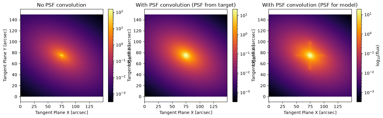
Extended model PSF convolution

For extended sources (galaxies mostly), an important part of astronomical image analysis is accounting for PSF effects. To that end, AstroPhot includes a number of approaches to handle PSF convolution. The main concept is that AstroPhot will convolve its model with a PSF before comparing against an image.

Note that psf_convolve is set to True by default, so if there is a PSF assigned to the model or its target then AstroPhot will try to convolve the model.

model_nopsf = ap.Model(
    model_type="sersic galaxy model",
    target=target,
    center=[75, 75],
    q=0.6,
    PA=60 * np.pi / 180,
    n=3,
    Re=10,
    Ie=10,
    psf_convolve=False,  # no PSF convolution will be done
)
model_nopsf.initialize()
model_psf = ap.Model(
    model_type="sersic galaxy model",
    target=target,
    center=[75, 75],
    q=0.6,
    PA=60 * np.pi / 180,
    n=3,
    Re=10,
    Ie=10,
    psf_convolve=True,  # now the PSF is convolved using the PSF from the target
)
model_psf.initialize()

psf = psf.copy()
psf[49:51] += 4 * np.mean(psf)
psf[:, 49:51] += 4 * np.mean(psf)
psf_target_2 = ap.PSFImage(
    data=psf,
    upsample=1,
)
psf_target_2.normalize()
model_selfpsf = ap.Model(
    model_type="sersic galaxy model",
    target=target,
    center=[75, 75],
    q=0.6,
    PA=60 * np.pi / 180,
    n=3,
    Re=10,
    Ie=10,
    psf=psf_target_2,  # Now this model has its own PSF, instead of using the target psf
)
model_selfpsf.initialize()

# With a convolved sersic the center is much more smoothed out
fig, ax = plt.subplots(1, 3, figsize=(15, 4))
ap.plots.model_image(fig, ax[0], model_nopsf)
ax[0].set_title("No PSF convolution")
ap.plots.model_image(fig, ax[1], model_psf)
ax[1].set_title("With PSF convolution (PSF from target)")
ap.plots.model_image(fig, ax[2], model_selfpsf)
ax[2].set_title("With PSF convolution (PSF for model)")
plt.show()

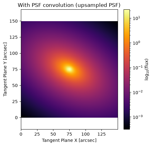
Supersampled PSF models

It is generally best practice to use a PSF model that has been determined at a higher resolution than the image you are analyzing. In AstroPhot this can be easily handled by setting the upsample value in a PSFImage to some integer greater than one. For example if our target has a pixelscale of 0.5 and the PSFImage has a pixelscale of 0.25 then you should set upsample=2 and AstroPhot model at 2x higher resolution.

upsample_psf_target = ap.PSFImage(
    data=ap.utils.initialize.gaussian_psf(2.0, 51, 0.25),
    upsample=2,  # This PSF is at 2x higher resolution than the target
)
target.psf = upsample_psf_target

model_upsamplepsf = ap.Model(
    model_type="sersic galaxy model",
    target=target,
    center=[75, 75],
    q=0.6,
    PA=60 * np.pi / 180,
    n=3,
    Re=10,
    Ie=10,
)
model_upsamplepsf.initialize()
fig, ax = plt.subplots(1, 1, figsize=(5, 5))
ap.plots.model_image(fig, ax, model_upsamplepsf)
ax.set_title("With PSF convolution (upsampled PSF)")
plt.show()

That covers the basics of adding PSF convolution kernels to AstroPhot models! These techniques assume you already have a model for the PSF that you got with some other algorithm (ie PSFEx), however AstroPhot also has the ability to model the PSF live along with the rest of the models in an image. If you are interested in extracting the PSF from an image using AstroPhot, check out the AdvancedPSFModels tutorial.