Aligning Images#
In AstroPhot, the image WCS is part of the model and so can be optimized alongside other model parameters. Here we will demonstrate a basic example of image alignment, but the sky is the limit, you can perform highly detailed image alignment with AstroPhot!
import astrophot as ap
import matplotlib.pyplot as plt
import numpy as np
import torch
from astropy.io import fits
Relative shift#
Often the WCS solution is already really good, we just need a local shift in x and/or y to get things just right. Lets start by optimizing a translation in the WCS that improves the fit for our models!
############ UNCOMMENT IF RUNNING LOCALLY ############
# hdu = fits.open(
# "https://www.legacysurvey.org/viewer/fits-cutout?ra=329.2715&dec=13.6483&size=150&layer=ls-dr9&pixscale=0.262&bands=r"
# )
# hdu.writeto("align_target_image_r.fits", overwrite=True)
# hdu = fits.open(
# "https://www.legacysurvey.org/viewer/fits-cutout?ra=329.2715&dec=13.6483&size=150&layer=ls-dr9&pixscale=0.262&bands=g"
# )
# hdu.writeto("align_target_image_g.fits", overwrite=True)
target_r = ap.TargetImage(
filename="align_target_image_r.fits",
name="target_r",
variance="auto",
)
target_g = ap.TargetImage(
filename="align_target_image_g.fits",
name="target_g",
variance="auto",
)
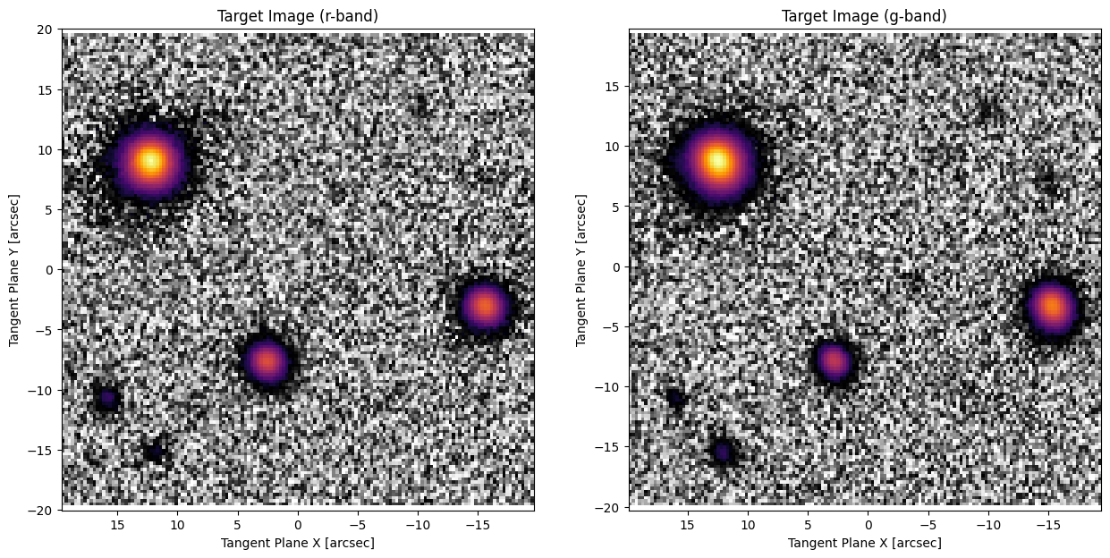
# Uh-oh! our images are misaligned by 1 pixel, this will cause problems!
target_g.crpix = target_g.crpix + 1
fig, axarr = plt.subplots(1, 2, figsize=(15, 7))
ap.plots.target_image(fig, axarr[0], target_r)
axarr[0].set_title("Target Image (r-band)")
ap.plots.target_image(fig, axarr[1], target_g)
axarr[1].set_title("Target Image (g-band)")
plt.show()
# fmt: off
# r-band model
psfr = ap.Model(name="psfr", model_type="moffat psf model", n=2, Rd=1.0, target=target_r.psf_image(data=np.zeros((51, 51))))
star1r = ap.Model(name="star1_r", model_type="point model", window=[0, 60, 80, 135], center=[12, 9], psf=psfr, target=target_r)
star2r = ap.Model(name="star2_r", model_type="point model", window=[40, 90, 20, 70], center=[3, -7], psf=psfr, target=target_r)
star3r = ap.Model(name="star3_r", model_type="point model", window=[109, 150, 40, 90], center=[-15, -3], psf=psfr, target=target_r)
modelr = ap.Model(name="model_r", model_type="group model", models=[star1r, star2r, star3r], target=target_r)
# g-band model
psfg = ap.Model(name="psfg", model_type="moffat psf model", n=2, Rd=1.0, target=target_g.psf_image(data=np.zeros((51, 51))))
star1g = ap.Model(name="star1_g", model_type="point model", window=[0, 60, 80, 135], center=star1r.center, psf=psfg, target=target_g)
star2g = ap.Model(name="star2_g", model_type="point model", window=[40, 90, 20, 70], center=star2r.center, psf=psfg, target=target_g)
star3g = ap.Model(name="star3_g", model_type="point model", window=[109, 150, 40, 90], center=star3r.center, psf=psfg, target=target_g)
modelg = ap.Model(name="model_g", model_type="group model", models=[star1g, star2g, star3g], target=target_g)
# total model
target_full = ap.TargetImageList([target_r, target_g])
model = ap.Model(name="model", model_type="group model", models=[modelr, modelg], target=target_full)
# fmt: on
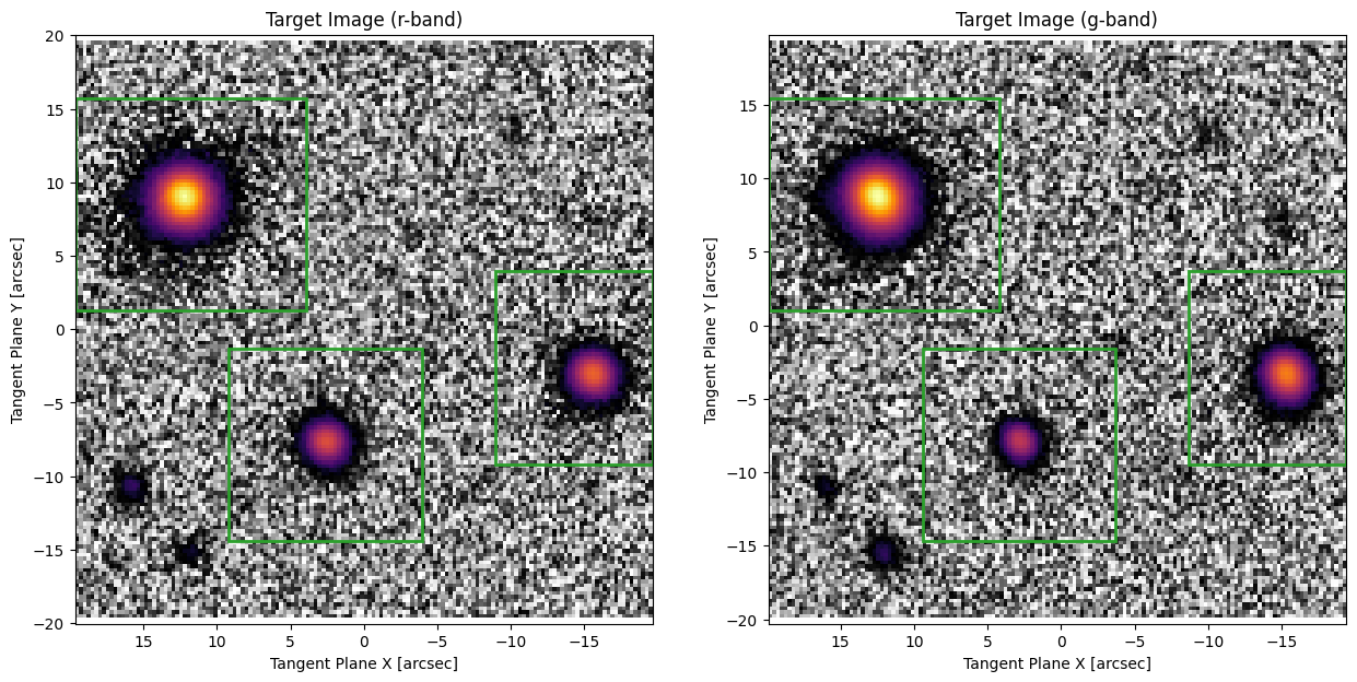
fig, axarr = plt.subplots(1, 2, figsize=(15, 7))
ap.plots.target_image(fig, axarr, target_full)
axarr[0].set_title("Target Image (r-band)")
axarr[1].set_title("Target Image (g-band)")
ap.plots.model_window(fig, axarr[0], modelr)
ap.plots.model_window(fig, axarr[1], modelg)
plt.show()
model.initialize()
res = ap.fit.LM(model, verbose=1).fit()
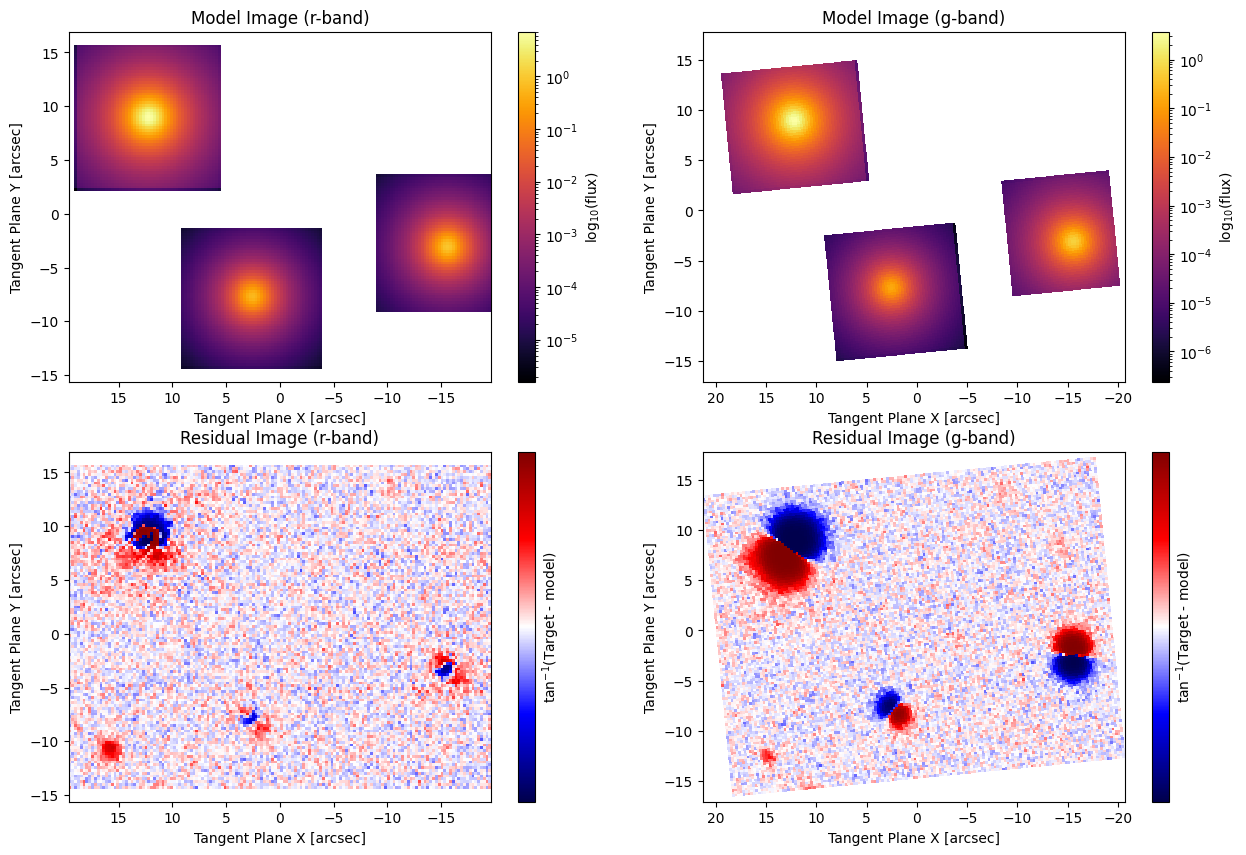
fig, axarr = plt.subplots(2, 2, figsize=(15, 10))
ap.plots.model_image(fig, axarr[0], model)
axarr[0, 0].set_title("Model Image (r-band)")
axarr[0, 1].set_title("Model Image (g-band)")
ap.plots.residual_image(fig, axarr[1], model)
axarr[1, 0].set_title("Residual Image (r-band)")
axarr[1, 1].set_title("Residual Image (g-band)")
plt.show()
Initializing model model_r
Initializing model star1_r
Initializing model star2_r
Initializing model star3_r
Initializing model model_g
Initializing model star1_g
Initializing model star2_g
Initializing model star3_g
==Starting LM fit for 'model' with 16 dynamic parameters and 34500 pixels==
Chi^2/DoF: 72.4148, L: 1
/home/docs/checkouts/readthedocs.org/user_builds/astrophot/envs/v0.17.2/lib/python3.12/site-packages/torch/jit/_script.py:1488: DeprecationWarning: `torch.jit.script` is deprecated. Please switch to `torch.compile` or `torch.export`.
  warnings.warn(
Chi^2/DoF: 13.2481, L: 1
Chi^2/DoF: 7.6234, L: 1
Chi^2/DoF: 6.21152, L: 1
Chi^2/DoF: 5.4456, L: 1
Chi^2/DoF: 3.88275, L: 0.111
Chi^2/DoF: 3.22983, L: 0.111
Chi^2/DoF: 2.78196, L: 0.0123
Chi^2/DoF: 2.66385, L: 0.000152
Chi^2/DoF: 2.65817, L: 1.88e-06
Chi^2/DoF: 2.65813, L: 1.88e-06
Final Chi^2/DoF: 2.65813, L: 2.32e-08. Converged: success
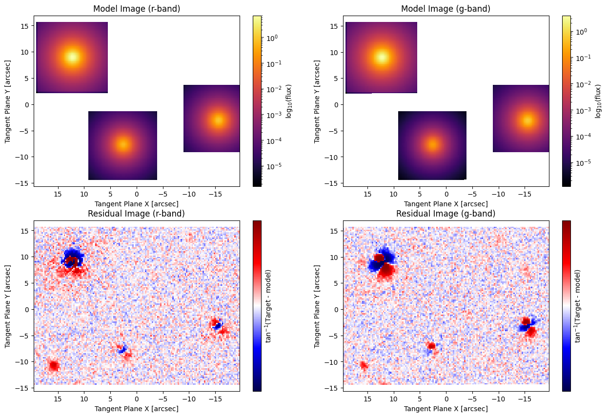
Here we see a clear signal of an image misalignment, in the g-band all of the residuals have a dipole in the same direction! Lets free up the position of the g-band image and optimize a shift. This only requires a single line of code!
target_g.crtan.to_dynamic()
Now we can optimize the model again, notice how it now has two more parameters. These are the x,y position of the image in the tangent plane. See the AstroPhot coordinate description on the website for more details on why this works.
res = ap.fit.LM(model, verbose=1).fit()
fig, axarr = plt.subplots(2, 2, figsize=(15, 10))
ap.plots.model_image(fig, axarr[0], model)
axarr[0, 0].set_title("Model Image (r-band)")
axarr[0, 1].set_title("Model Image (g-band)")
ap.plots.residual_image(fig, axarr[1], model)
axarr[1, 0].set_title("Residual Image (r-band)")
axarr[1, 1].set_title("Residual Image (g-band)")
plt.show()
==Starting LM fit for 'model' with 18 dynamic parameters and 34500 pixels==
Chi^2/DoF: 2.65828, L: 1
Chi^2/DoF: 2.05093, L: 1
Chi^2/DoF: 1.7765, L: 1
Chi^2/DoF: 1.55578, L: 0.111
Chi^2/DoF: 1.53732, L: 1.69e-05
Chi^2/DoF: 1.53715, L: 1.88e-06
Chi^2/DoF: 1.53707, L: 3.33
Chi^2/DoF: 1.53707, L: 403
Chi^2/DoF: 1.53707, L: 403
Chi^2/DoF: 1.53707, L: 403
Chi^2/DoF: 1.53707, L: 403
Chi^2/DoF: 1.53707, L: 403
Chi^2/DoF: 1.53707, L: 403
Chi^2/DoF: 1.53707, L: 403
Chi^2/DoF: 1.53707, L: 403
Chi^2/DoF: 1.53707, L: 403
Chi^2/DoF: 1.53707, L: 403
Chi^2/DoF: 1.53707, L: 403
Chi^2/DoF: 1.53707, L: 403
Final Chi^2/DoF: 1.53707, L: 403. Converged: success by immobility. Convergence not guaranteed

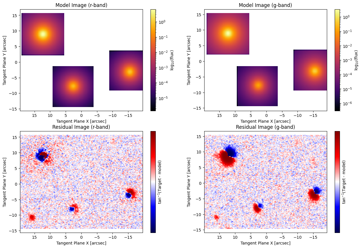
Yay! no more dipole. The fits aren’t the best, clearly these objects aren’t super well described by a single moffat model. But the main goal today was to show that we could align the images very easily. Note, its probably best to start with a reasonably good WCS from the outset, and this two stage approach where we optimize the models and then optimize the models plus a shift might be more stable than just fitting everything at once from the outset. Often for more complex models it is best to start with a simpler model and fit each time you introduce more complexity.
Shift and rotation#
Lets say we really don’t trust our WCS, we think something has gone wrong and we want freedom to fully shift and rotate the relative positions of the images relative to each other. How can we do this?
def rotate(phi):
    """Create a 2D rotation matrix for a given angle in radians."""
    return torch.stack(
        [
            torch.stack([torch.cos(phi), -torch.sin(phi)]),
            torch.stack([torch.sin(phi), torch.cos(phi)]),
        ]
    )


# Uh-oh! Our image is misaligned by some small angle
target_g.CD = target_g.CD.value @ rotate(torch.tensor(np.pi / 32, dtype=torch.float64))
# Uh-oh! our alignment from before has been erased
target_g.crtan.value = (0, 0)
fig, axarr = plt.subplots(2, 2, figsize=(15, 10))
ap.plots.model_image(fig, axarr[0], model)
axarr[0, 0].set_title("Model Image (r-band)")
axarr[0, 1].set_title("Model Image (g-band)")
ap.plots.residual_image(fig, axarr[1], model)
axarr[1, 0].set_title("Residual Image (r-band)")
axarr[1, 1].set_title("Residual Image (g-band)")
plt.show()
Notice that there is not a universal dipole like in the shift example. Most of the offset is caused by the rotation in this example.
# this will control the relative rotation of the g-band image
phi = ap.Param(name="phi", value=0.0, dynamic=True, dtype=torch.float64)

# Set the target_g CD matrix to be a function of the rotation angle
# The CD matrix can encode rotation, skew, and rectangular pixels. We
# are only interested in the rotation here.
init_CD = target_g.CD.value.clone()
target_g.CD = lambda p: init_CD @ rotate(p.phi.value)
target_g.CD.link(phi)

# also optimize the shift of the g-band image
target_g.crtan.to_dynamic()
res = ap.fit.LM(model, verbose=1).fit()
fig, axarr = plt.subplots(2, 2, figsize=(15, 10))
ap.plots.model_image(fig, axarr[0], model)
axarr[0, 0].set_title("Model Image (r-band)")
axarr[0, 1].set_title("Model Image (g-band)")
ap.plots.residual_image(fig, axarr[1], model)
axarr[1, 0].set_title("Residual Image (r-band)")
axarr[1, 1].set_title("Residual Image (g-band)")
plt.show()
==Starting LM fit for 'model' with 19 dynamic parameters and 34500 pixels==
Chi^2/DoF: 171.084, L: 1
Chi^2/DoF: 31.2056, L: 1
Chi^2/DoF: 9.70858, L: 1
Chi^2/DoF: 5.62903, L: 1
Chi^2/DoF: 4.07284, L: 1
Chi^2/DoF: 2.82666, L: 1
Chi^2/DoF: 2.24942, L: 1
Chi^2/DoF: 1.73518, L: 0.111
Chi^2/DoF: 1.5431, L: 0.0123
Chi^2/DoF: 1.53439, L: 0.000152
Chi^2/DoF: 1.53437, L: 24.5
Chi^2/DoF: 1.53436, L: 24.5
Chi^2/DoF: 1.53436, L: 270
Chi^2/DoF: 1.53434, L: 30
Chi^2/DoF: 1.53434, L: 330
Could not find step to improve Chi^2, stopping
Final Chi^2/DoF: 1.53434, L: 330. Converged: success by immobility. Could not find step to improve Chi^2. Convergence not guaranteed