Custom model objects

Here we will go over some of the core functionality of AstroPhot models so that you can make your own custom models with arbitrary behavior. This is an advanced tutorial and likely not needed for most users. However, the flexibility of AstroPhot can be a real lifesaver for some niche applications! If you get stuck trying to make your own models, please contact Connor Stone (see GitHub), he can help you get the model working and maybe even help add it to the core AstroPhot model list!

AstroPhot model hierarchy

AstroPhot models are very much object oriented and inheritance driven. Every AstroPhot model inherits from Model and so if you wish to make something truly original then this is where you would need to start. However, it is almost certain that is the wrong way to go. Further down the hierarchy is the ComponentModel object, this is what you will likely use to construct a custom model as it represents a single “unit” in the astronomical image. Spline, Sersic, Exponential, Gaussian, PSF, Sky, etc. all of these inherit from ComponentModel so likely that’s what you will want. At its core, a ComponentModel object defines a center location for the model, but it doesn’t know anything else yet. At the same level as ComponentModel is GroupModel which represents a collection of model objects (typically but not always ComponentModel objects). A GroupModel is how you construct more complex models by composing several simpler models. It’s unlikely you’ll need to inherit from GroupModel so we won’t discuss this any further (contact the developers if you’re thinking about that).

Inheriting from ComponentModel are a few general classes which make it easier to build typical cases. There is the GalaxyModel which adds a position angle and axis ratio to the model; also PointSource which simply enforces some restrictions that make more sense for a delta function model; SkyModel should be used for anything low resolution defined over the entire image, in this model psf convolution and sub-pixel integration are turned off since they shouldn’t be needed. Based on these low level classes, you can “jump in” where it makes sense to define your model. If you are looking to define a sersic that has some slightly different behaviour you may be able to take the SersicGalaxy class and directly make your modification. Of course, you can take any AstroPhot model as a starting point and modify it to suit a given task, however we will not list all models here. See the documentation for a more complete list.

Remaking the Sersic model

Here we will remake the sersic model in AstroPhot to demonstrate how new models can be created

import astrophot as ap
import torch
from astropy.io import fits
import numpy as np
import matplotlib.pyplot as plt

class My_Sersic(ap.models.RadialMixin, ap.models.GalaxyModel):
    """Let's make a sersic model!"""

    _model_type = "mysersic"  # here we give a name to the model, since we inherit from GalaxyModel the full model_type will be "mysersic galaxy model"
    _parameter_specs = {
        # our sersic index will have some default limits so it doesn't produce
        # weird results We also indicate the expected shapeof the parameter, in
        # this case a scalar. This isn't necessary but it gives AstroPhot more
        # information to work with. if e.g. you accidentaly provide multiple
        # values, you'll now get an error rather than confusing behavior later.
        "my_n": {"valid": (0.36, 8), "shape": (), "dynamic": True},
        "my_Re": {"units": "arcsec", "valid": (0, None), "shape": (), "dynamic": True},
        "my_Ie": {"units": "flux/arcsec^2", "dynamic": True},
    }

    # a GalaxyModel object will determine the radius for each pixel then call radial_model to determine the brightness
    @ap.forward
    def radial_model(self, R, my_n, my_Re, my_Ie):
        bn = ap.models.func.sersic_n_to_b(my_n)
        return my_Ie * torch.exp(-bn * ((R / my_Re) ** (1.0 / my_n) - 1))

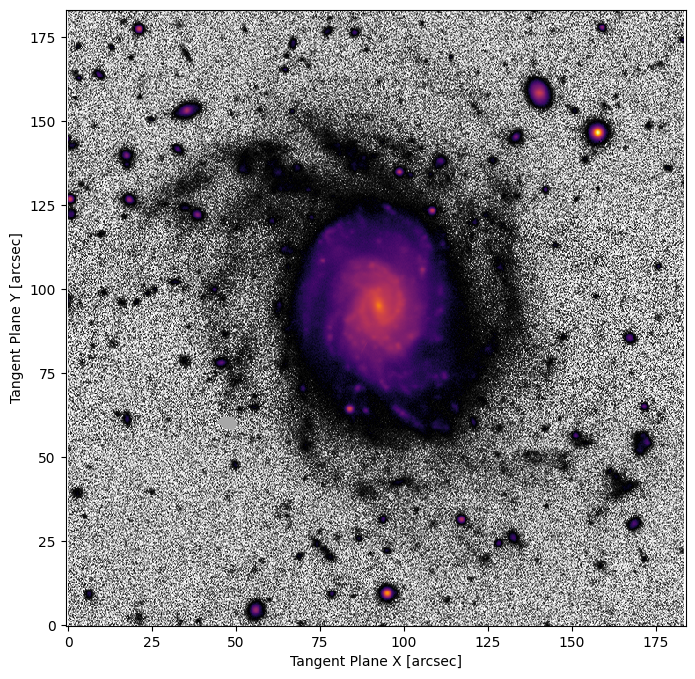
Now lets try optimizing our sersic model on some data. We’ll use the same galaxy from the GettingStarted tutorial. The results should be about the same!

############# UNCOMMENT IF RUNNING LOCALLY ############
# hdu = fits.open(
#     "https://www.legacysurvey.org/viewer/fits-cutout?ra=36.3684&dec=-25.6389&size=700&layer=ls-dr9&pixscale=0.262&bands=r"
# )
hdu = fits.open("target_image.fits")
target_data = np.array(hdu[0].data, dtype=np.float64)

target = ap.TargetImage(data=target_data, pixelscale=0.262, zeropoint=22.5, variance="auto")

fig, ax = plt.subplots(figsize=(8, 8))
ap.plots.target_image(fig, ax, target)
plt.show()

my_model = My_Sersic(  # notice we are now using the custom class
    name="wow_I_made_a_model",
    target=target,  # now the model knows what its trying to match
    # note we have to give initial values for our new parameters. AstroPhot doesn't know how to auto-initialize them because they are custom
    my_n=1.0,
    my_Re=50,
    my_Ie=1.0,
)

# We gave it parameters for our new variables, but initialize will get starting values for everything else
my_model.initialize()

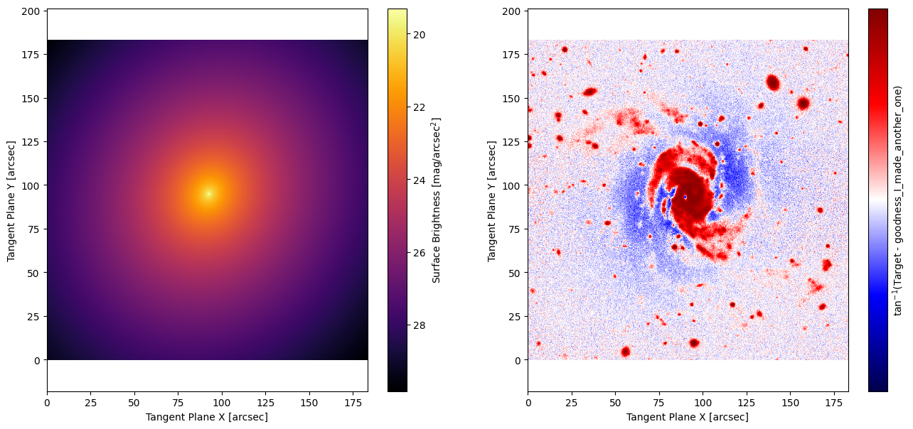
# The starting point for this model is not very good, lets see what the optimizer can do!
fig, ax = plt.subplots(1, 2, figsize=(16, 7))
ap.plots.model_image(fig, ax[0], my_model)
ap.plots.residual_image(fig, ax[1], my_model)
plt.show()

result = ap.fit.LM(my_model, verbose=1).fit()
print(result.message)

==Starting LM fit for 'wow_I_made_a_model' with 7 dynamic parameters and 490000 pixels==

Chi^2/DoF: 496.215, L: 1

/home/docs/checkouts/readthedocs.org/user_builds/astrophot/envs/v0.17.0/lib/python3.12/site-packages/torch/jit/_script.py:1488: DeprecationWarning: `torch.jit.script` is deprecated. Please switch to `torch.compile` or `torch.export`.
  warnings.warn(

Chi^2/DoF: 47.8174, L: 1

Chi^2/DoF: 18.9797, L: 1

Chi^2/DoF: 13.7514, L: 1

Chi^2/DoF: 10.6755, L: 1

Chi^2/DoF: 8.77446, L: 0.111

Chi^2/DoF: 8.0632, L: 0.0123

Chi^2/DoF: 7.15818, L: 0.0123

Chi^2/DoF: 6.73283, L: 0.0123

Chi^2/DoF: 6.71174, L: 2.32e-08

Chi^2/DoF: 6.71121, L: 2.32e-08

Final Chi^2/DoF: 6.7112, L: 2.32e-08. Converged: success

success

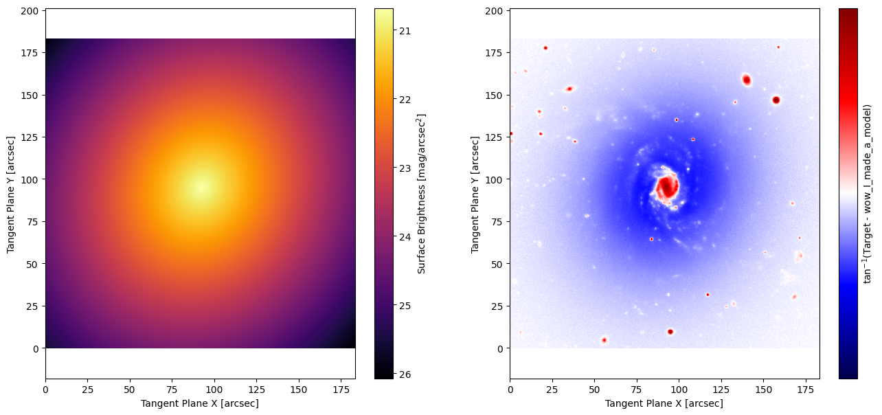
fig, ax = plt.subplots(1, 2, figsize=(16, 7))
ap.plots.model_image(fig, ax[0], my_model)
ap.plots.residual_image(fig, ax[1], my_model)
plt.show()

Success! Our “custom” sersic model behaves exactly as expected. While going through the tutorial so far there may have been a few things that stood out to you. Lets discuss them now:

• What is ap.models.RadialMixin? Think of “Mixin’s” as power ups for classes, this power up makes a brightness function which calls radial_model to determine the flux density, that way you only need to define a radial function rather than a more general brightness(x,y) 2D function.

• what else is in “ap.models.func”? Lots of stuff used in the background by AstroPhot models. There is a similar ap.image.func for image specific functions. You can use these, or write your own functions.

• How did the radial_model function accept the parameters I defined in _parameter_specs? That’s the work of caskade a powerful parameter management tool.

• When making the model, why did we have to provide values for the parameters? Every model can define an “initialize” function which sets the values for its parameters. Since we didn’t add that function to our custom class, it doesn’t know how to set those variables. All the other variables can be auto-initialized though.

• Why is radial_model decorated with @ap.forward? This is part of the caskade system, the @ap.forward here does a lot of heavily lifting automatically to fill in values for my_n, my_Re, and my_Ie

Adding an initialize method

Here we’ll add an initialize method. Though for simplicity we won’t make it very clever. It will be up to you to figure out the best way to start your parameters. The initial values can have a huge impact on how well the model converges to the solution, so don’t underestimate the gains that can be made by thinking a bit about how to do this right. The default AstroPhot methods have reasonably robust initializers, but still nothing beats trial and error by eye to get started.

# note we're inheriting everything from the My_Sersic model since its not making any new parameters
class My_Super_Sersic(My_Sersic):
    _model_type = "super"  # the new name will be "super mysersic galaxy model"

    def initialize(self):
        # typically you want all the lower level parameters determined first
        super().initialize()

        # this gets the part of the image that the user actually wants us to analyze
        target_area = target[self.window]

        # only initialize if the user didn't already provide a value
        if not self.my_n.initialized:
            # make an initial value for my_n. It's a "dynamic_value" so it can be optimized later
            self.my_n.value = 2.0

        if not self.my_Re.initialized:
            self.my_Re.value = 20.0

        # lets try to be a bit clever here. This will be an average in the
        # window, should at least get us within an order of magnitude
        if not self.my_Ie.initialized:
            center = target_area.plane_to_pixel(*self.center.value)
            i, j = int(center[0].item()), int(center[1].item())
            self.my_Ie.value = (
                torch.median(target_area.data[i - 100 : i + 100, j - 100 : j + 100])
                / target_area.pixel_area
            )

my_super_model = ap.Model(
    name="goodness_I_made_another_one",
    model_type="super mysersic galaxy model",  # this is the type we defined above
    target=target,
)

my_super_model.initialize()

# The starting point for this model is still not very good, lets see what the optimizer can do!
fig, ax = plt.subplots(1, 2, figsize=(16, 7))
ap.plots.model_image(fig, ax[0], my_super_model)
ap.plots.residual_image(fig, ax[1], my_super_model)
plt.show()

# We made a "good" initializer so this should be faster to optimize
result = ap.fit.LM(my_super_model, verbose=1).fit()
print(result.message)

==Starting LM fit for 'goodness_I_made_another_one' with 7 dynamic parameters and 490000 pixels==

Chi^2/DoF: 8.7962, L: 1

Chi^2/DoF: 7.78726, L: 0.111

Chi^2/DoF: 7.53067, L: 0.111

Chi^2/DoF: 6.99031, L: 0.0123

Chi^2/DoF: 6.73562, L: 0.0123

Chi^2/DoF: 6.71168, L: 2.32e-08

Chi^2/DoF: 6.71121, L: 2.32e-08

Final Chi^2/DoF: 6.7112, L: 2.32e-08. Converged: success

success

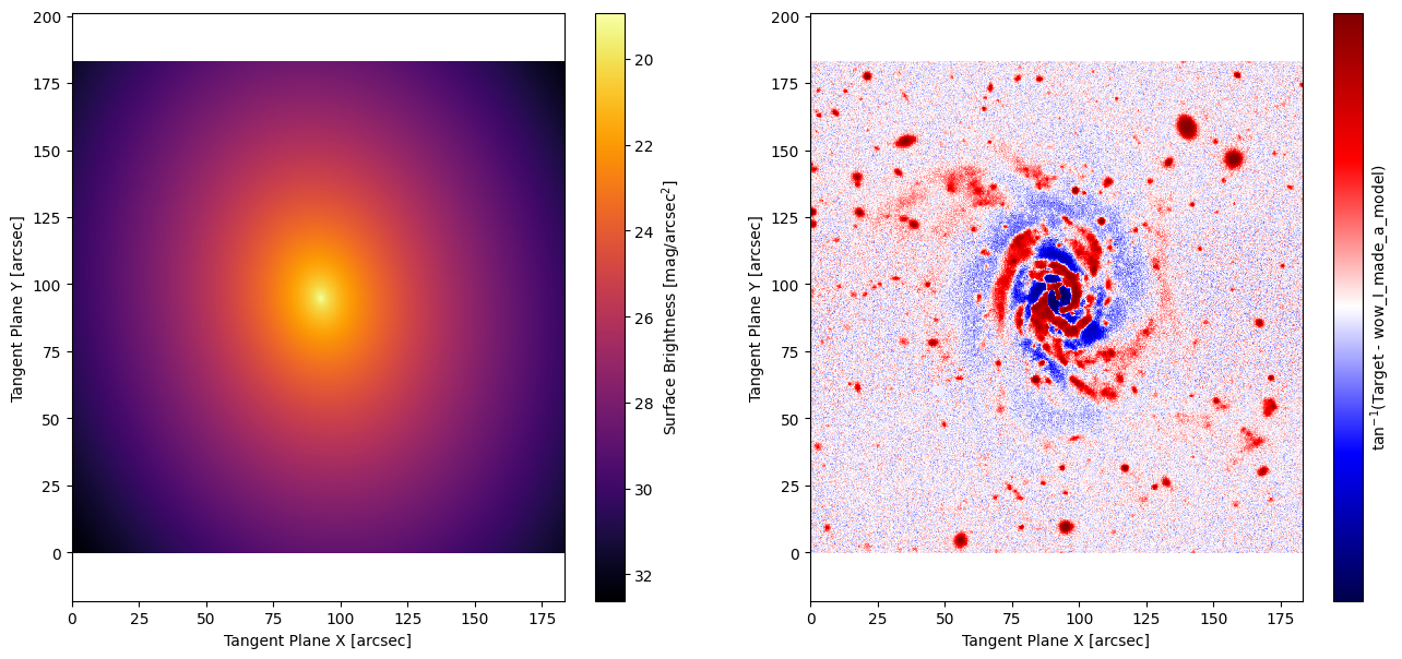
fig, ax = plt.subplots(1, 2, figsize=(16, 7))
ap.plots.model_image(fig, ax[0], my_super_model)
ap.plots.residual_image(fig, ax[1], my_super_model)
plt.show()

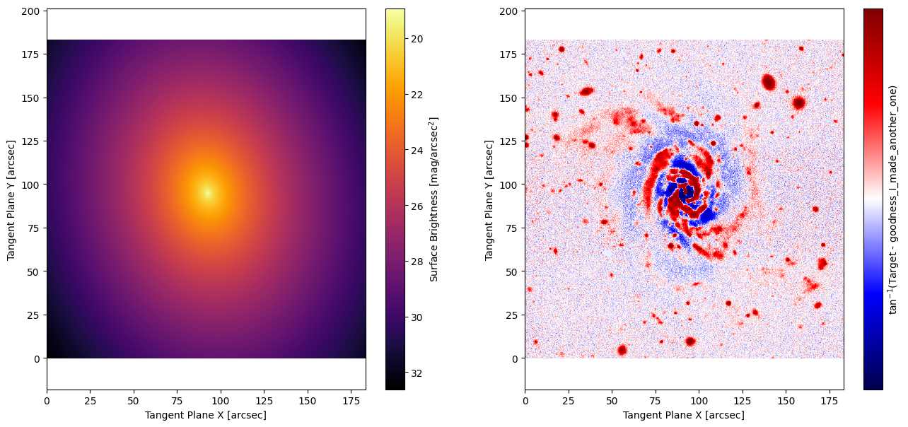
Success! That covers the basics of making your own models. There’s an infinite amount of possibility here so you will likely need to hunt through the AstroPhot code to find answers to more nuanced questions (or contact Connor), but hopefully this tutorial gave you a flavour of what to expect.

Models from scratch

By inheriting from GalaxyModel we got to start with some methods already available. In this section we will see how to create a model essentially from scratch by inheriting from the ComponentModel object. Below is an example model which uses a \(\frac{I_0}{R}\) model, this is a weird model but it will work. To demonstrate the basics for a ComponentModel is actually simpler than a GalaxyModel we really only need the brightness(x,y) function, it’s what you do with that function where the complexity arises.

class My_InvR(ap.models.ComponentModel):
    _model_type = "InvR"

    _parameter_specs = {
        # scale length
        "my_Rs": {"units": "arcsec", "valid": (0, None)},
        "my_I0": {"units": "flux/arcsec^2"},  # central brightness
    }

    def __init__(self, *args, epsilon=1e-4, **kwargs):
        super().__init__(*args, **kwargs)
        self.epsilon = epsilon

    @ap.forward
    def brightness(self, x, y, my_Rs, my_I0):
        x, y = self.transform_coordinates(
            x, y
        )  # basically just subtracts the center from the coordinates
        R = torch.sqrt(x**2 + y**2 + self.epsilon) / my_Rs
        return my_I0 / R

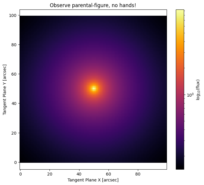
See now that we must define a brightness method. This takes general tangent plane coordinates and returns the model evaluated at those coordinates. No need to worry about integrating the model within a pixel, this will be handled internally, just evaluate the model at exactly the coordinates requested. We also add a new value epsilon which is a core radius in arcsec and stops numerical divide by zero errors at the center. This parameter will not be fit, it is set as part of the model creation. You can now also provide epsilon when creating the model, or do nothing and the default value will be used.

From here you have complete freedom, make sure to use only pytorch functions, since that way it is possible to run on GPU and propagate derivatives.

simpletarget = ap.TargetImage(data=np.zeros([100, 100]), pixelscale=1)
newmodel = ap.Model(
    name="newmodel",
    model_type="InvR model",  # this is the type we defined above
    epsilon=1,
    center=[50, 50],
    my_Rs=10,
    my_I0=1.0,
    target=simpletarget,
)

fig, ax = plt.subplots(1, 1, figsize=(8, 7))
ap.plots.model_image(fig, ax, newmodel)
ax.set_title("Observe parental-figure, no hands!")
plt.show()