Gravitational Lensing#
AstroPhot is now part of the caskade ecosystem. caskade simulators can interface very easily since the parameter management is handled automatically. Here we demonstrate how the caustics package, which is also written in caskade, can be used to add gravitational lensing to AstroPhot models. This is similar to the Custom Models tutorial although more specific.
import astrophot as ap
import matplotlib.pyplot as plt
import caustics
import numpy as np
import torch
from astropy.io import fits
class LensSersic(ap.models.SersicGalaxy):
    _model_type = "lensed"

    def __init__(self, *args, lens, **kwargs):
        super().__init__(*args, **kwargs)
        self.lens = lens

    def transform_coordinates(self, x, y):
        x, y = self.lens.raytrace(x, y)
        x, y = super().transform_coordinates(x, y)
        return x, y
############ UNCOMMENT IF RUNNING LOCALLY ############
# hdu = fits.open(
#     "https://www.legacysurvey.org/viewer/fits-cutout?ra=177.1380&dec=19.5008&size=150&layer=ls-dr9&pixscale=0.262&bands=g"
# )
# hdu.writeto("lensed_target_image.fits", overwrite=True)
target = ap.TargetImage(
    filename="lensed_target_image.fits",
    name="horseshoe",
    variance="auto",
    zeropoint=22.5,
)
target.psf = target.psf_image(data=ap.utils.initialize.gaussian_psf(0.5, 51, 0.262))

cosmology = caustics.FlatLambdaCDM(name="cosmology")
lens = caustics.SIE(
    name="lens",
    x0=0.28,
    y0=0.79,
    q=0.9,
    phi=2.5 * np.pi / 10,
    Rein=5.5,
    z_l=0.4457,
    z_s=2.379,
    cosmology=cosmology,
)
lens.to_dynamic()
lens.z_l.to_static()
lens.z_s.to_static()
source = ap.Model(
    name="source",
    model_type="lensed sersic galaxy model",
    lens=lens,
    center=[0.2, 0.42],
    q=0.6,
    PA=np.pi / 3,
    n=1,
    Re=0.1,
    Ie=1.5,
    target=target,
    psf_convolve=True,
)
lenslight = ap.Model(
    name="lenslight",
    model_type="sersic galaxy model",
    center=lambda p: torch.stack((p.x0.value, p.y0.value)),
    q=lens.q,
    PA=0,
    n=4.7,
    Re=1,
    Ie=0.2,
    target=target,
    psf_convolve=True,
)
lenslight.center.link((lens.x0, lens.y0))

model = ap.Model(
    name="horseshoe",
    model_type="group model",
    models=[source, lenslight],
    target=target,
)
model.initialize()

fig, axarr = plt.subplots(1, 3, figsize=(15, 4))
ap.plots.target_image(fig, axarr[0], target)
axarr[0].set_title("Target Image")
ap.plots.model_image(fig, axarr[1], model)
axarr[1].set_title("Model Image")
ap.plots.residual_image(fig, axarr[2], model)
axarr[2].set_title("Residual Image")
plt.show()
Initializing model source
Initializing model lenslight
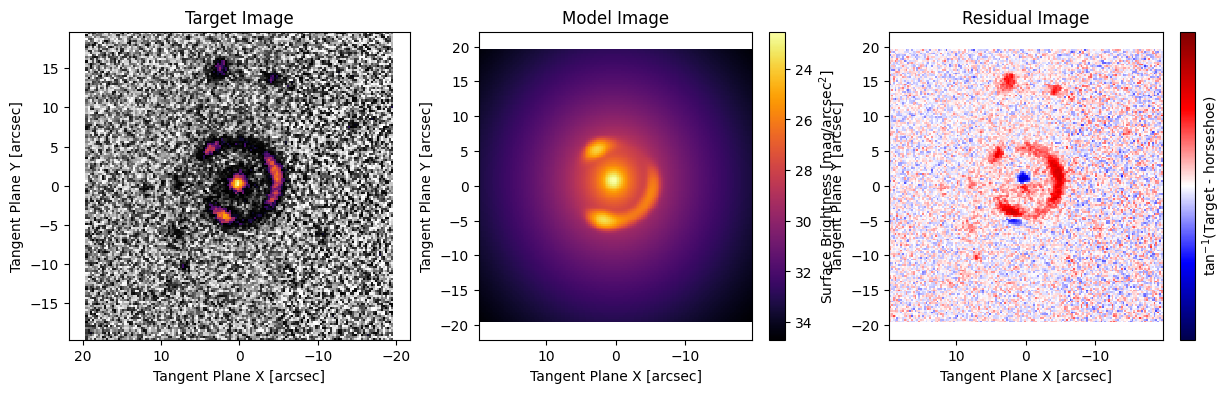
Note that we give reasonable starting parameters for the lensing model. Gravitational lensing is notoriously hard to model, so we need to start near the correct minimum otherwise we may easily fall to some poor local minimum.
model.graphviz()

res = ap.fit.LM(model, verbose=1).fit()
==Starting LM fit for 'horseshoe' with 16 dynamic parameters and 22500 pixels==
Chi^2/DoF: 5.09753, L: 1
/home/docs/checkouts/readthedocs.org/user_builds/astrophot/envs/v0.17.0/lib/python3.12/site-packages/torch/jit/_script.py:1488: DeprecationWarning: `torch.jit.script` is deprecated. Please switch to `torch.compile` or `torch.export`.
  warnings.warn(
Chi^2/DoF: 4.85478, L: 0.111
Chi^2/DoF: 4.78083, L: 0.111
Chi^2/DoF: 4.74452, L: 0.111
Chi^2/DoF: 4.74139, L: 0.0123
Chi^2/DoF: 4.74051, L: 0.136
Chi^2/DoF: 4.73887, L: 0.0151
Chi^2/DoF: 4.73721, L: 0.0151
Chi^2/DoF: 4.73671, L: 0.0151
Chi^2/DoF: 4.73635, L: 0.0151
Chi^2/DoF: 4.7359, L: 0.0151
Chi^2/DoF: 4.73505, L: 0.166
Chi^2/DoF: 4.73487, L: 1.83
Chi^2/DoF: 4.73475, L: 20.1
Chi^2/DoF: 4.73467, L: 20.1
Chi^2/DoF: 4.73463, L: 20.1
Chi^2/DoF: 4.73461, L: 20.1
Chi^2/DoF: 4.7346, L: 20.1
Chi^2/DoF: 4.73459, L: 2.23
Chi^2/DoF: 4.73458, L: 24.5
Chi^2/DoF: 4.73458, L: 2.73
Chi^2/DoF: 4.73457, L: 2.73
Chi^2/DoF: 4.73456, L: 2.73
Chi^2/DoF: 4.73456, L: 2.73
Chi^2/DoF: 4.73455, L: 2.73
Chi^2/DoF: 4.73454, L: 2.73
Chi^2/DoF: 4.73454, L: 2.73
Chi^2/DoF: 4.73453, L: 2.73
Chi^2/DoF: 4.73322, L: 0.00374
Chi^2/DoF: 4.73269, L: 0.00374
Chi^2/DoF: 4.73161, L: 0.0412
Chi^2/DoF: 4.7314, L: 4.98
Chi^2/DoF: 4.73133, L: 4.98
Chi^2/DoF: 4.73129, L: 4.98
Chi^2/DoF: 4.73129, L: 603
Chi^2/DoF: 4.73129, L: 6.63e+03
Chi^2/DoF: 4.73129, L: 6.63e+03
Chi^2/DoF: 4.73129, L: 6.63e+03
Chi^2/DoF: 4.73129, L: 6.63e+03
Chi^2/DoF: 4.73129, L: 6.63e+03
Chi^2/DoF: 4.73129, L: 6.63e+03
Final Chi^2/DoF: 4.73129, L: 6.63e+03. Converged: success by immobility. Convergence not guaranteed
fig, axarr = plt.subplots(1, 3, figsize=(15, 4))
ap.plots.target_image(fig, axarr[0], target)
axarr[0].set_title("Target Image")
ap.plots.model_image(fig, axarr[1], model, vmax=32)
axarr[1].set_title("Model Image")
ap.plots.residual_image(fig, axarr[2], model)
axarr[2].set_title("Residual Image")
plt.show()
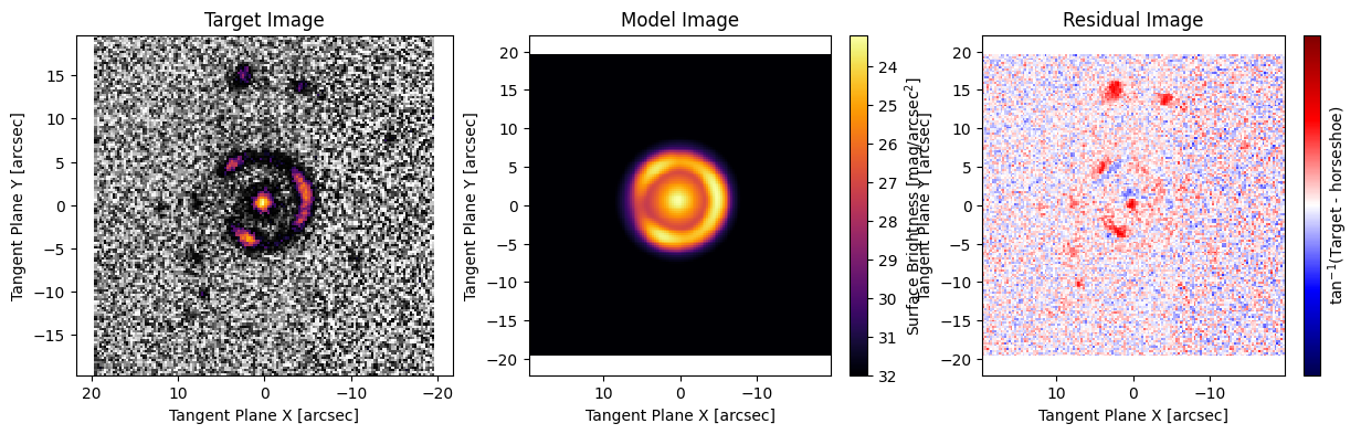
This is not an exceptionally good fit, but it is well known that the horseshoe requires a more detailed model than an SIE lens. The cool result here is that we were able to link AstroPhot and caustics very easily to create a detailed lensing model!