Functional AstroPhot interface#
AstroPhot is an object oriented code, meaning that it is build on python objects that behave in intuitively meaningful ways. For example it is possible to add two model images together to get a new model image, even if one of them only fills a subwindow of pixels, this is because the model images are aware of what part of the scene they represent and can behave accordingly. This is all very nice so long as you are building the kinds of models that AstroPhot is designed for, and when you are not trying to squeeze out every last bit of performance. For most cases, AstroPhot objects can handle complex configurations and perform very quickly. Still, you may need to push things with highly specific customization. Let’s consider a case where some specialization can give a big performance boost, a supernova light curve.
%matplotlib inline
%load_ext autoreload
%autoreload 2

import astrophot as ap
import numpy as np
import jax
import jax.numpy as jnp
import matplotlib.pyplot as plt
from corner import corner

ap.backend.backend = "jax"
Generate Mock data#
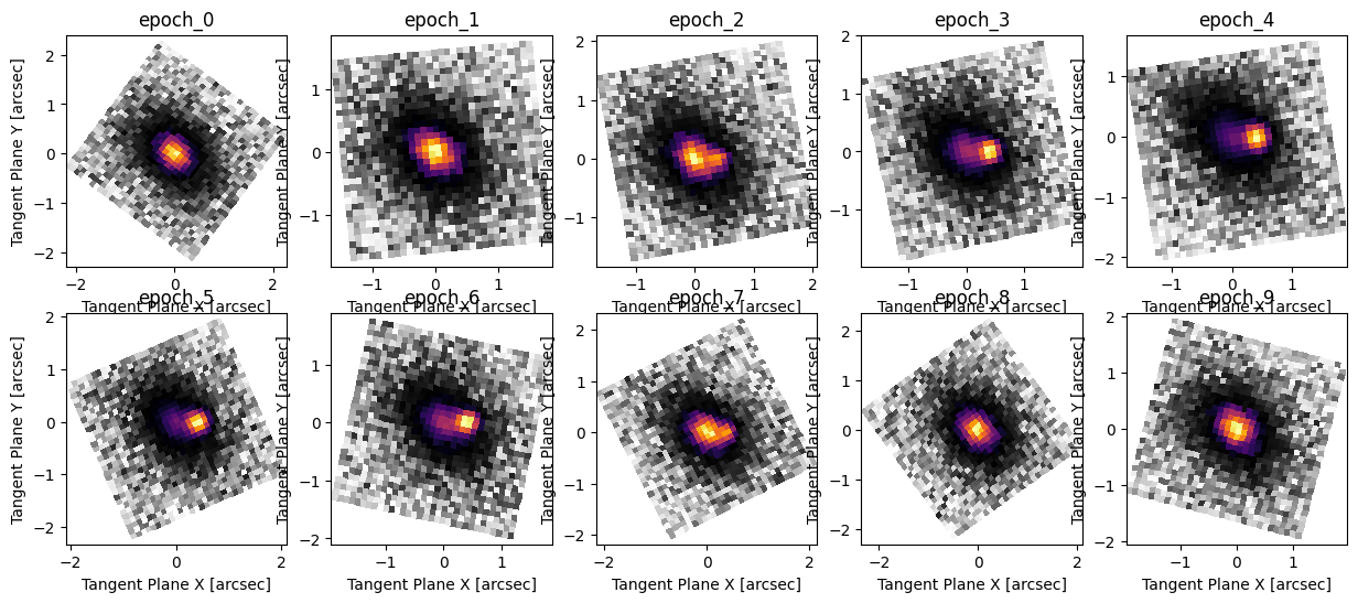
Here we will use the usual AstroPhot object oriented interface to generate some mock SN data. There is a fixed host Sersic galaxy, and a Gaussian point source with variable flux as the SN. Every observation is a new pointing of the telescope, so the images are not all aligned and are rotated randomly. The AstroPhot object oriented framework handles this by having target images aware of the WCS that connects the pixels to their location on the sky. We will see in the functional version that everything has to be more explicit, but is more or less the same.
INFO:2026-03-25 15:03:24,667:jax._src.xla_bridge:830: Unable to initialize backend 'tpu': INTERNAL: Failed to open libtpu.so: libtpu.so: cannot open shared object file: No such file or directory
Unable to initialize backend 'tpu': INTERNAL: Failed to open libtpu.so: libtpu.so: cannot open shared object file: No such file or directory
Build the functional model#
Below we build a functional version of the AstroPhot model which generated the data. The end result is an identical sampling algorithm which strips away all the object oriented layers of the AstroPhot model to give a pure function to compute pixel values. This is a very insightful exercise to learn exactly what AstroPhot does under the hood. As you can see, there are a number of subtle effects to account for which AstroPhot does automatically, but at a high level it is all very straightforward.
def model_img(
    sersic_x,
    sersic_y,
    sersic_q,
    sersic_PA,
    sersic_n,
    sersic_Re,
    sersic_Ie,
    psf,
    sn_x,
    sn_y,
    sn_flux,
    sky,
    crpix,
    crtan,
    CD,
):
    # Sample sersic
    pixel_area = 0.1 * 0.1
    # Pad by 20 pixels (10 on each side) to avoid edge effects from convolution
    i, j, w = ap.image.func.pixel_quad_meshgrid(
        (0, 32, 0, 32), 10, 1, ap.config.DTYPE, ap.config.DEVICE, order=3
    )
    #
    x, y = ap.image.func.pixel_to_plane_linear(j, i, *crpix, CD, *crtan)
    sx, sy = x - sersic_x, y - sersic_y
    sx, sy = ap.models.func.rotate(-sersic_PA + np.pi / 2, sx, sy)
    sy = sy / sersic_q
    sr = jnp.sqrt(sx**2 + sy**2)
    z = ap.models.func.sersic(sr, n=sersic_n, Re=sersic_Re, Ie=sersic_Ie)
    sample = ap.models.func.pixel_quad_integrator(z, w)
    sample = ap.models.func.convolve(sample, psf)
    sample = sample[10:-10, 10:-10] * pixel_area

    # Sample point source (empirical PSF)
    i, j, w = ap.image.func.pixel_quad_meshgrid(
        (0, 32, 0, 32), 0, 1, ap.config.DTYPE, ap.config.DEVICE, order=3
    )
    gj, gi = ap.image.func.plane_to_pixel_linear(sn_x, sn_y, *crpix, CD, *crtan)
    z = ap.utils.interpolate.interp2d(
        psf, j - gj + (psf.shape[1] // 2), i - gi + (psf.shape[0] // 2)
    )
    sample = sample + sn_flux * ap.models.func.pixel_quad_integrator(z, w)

    # add sky level
    return sample + sky


# fixed: sersic_x, sersic_y, psf, crpix, CD
# global: sersic_q, sersic_PA, sersic_n, sersic_Re, sersic_Ie, sn_x, sn_y
# per image: sky, sn_sigma, sn_flux, crtan


@jax.jit
def full_model(
    sersic_x,
    sersic_y,
    sersic_q,
    sersic_PA,
    sersic_n,
    sersic_Re,
    sersic_Ie,
    psf,
    sn_x,
    sn_y,
    sn_flux,
    sky,
    crpix,
    crtan,
    CD,
):
    return jax.vmap(
        model_img,
        in_axes=(None, None, None, None, None, None, None, None, None, None, 0, 0, 0, 0, 0),
    )(
        sersic_x,
        sersic_y,
        sersic_q,
        sersic_PA,
        sersic_n,
        sersic_Re,
        sersic_Ie,
        psf,
        sn_x,
        sn_y,
        sn_flux,
        sky,
        crpix,
        crtan,
        CD,
    )


def model(params, sersic_x, sersic_y, psf, crpix, CD):
    return full_model(
        sersic_x,
        sersic_y,
        params[0],
        params[1],
        params[2],
        params[3],
        params[4],
        psf,
        params[5],
        params[6],
        params[7:17],
        params[17:27],
        crpix,
        params[27:47].reshape(10, 2),
        CD,
    )
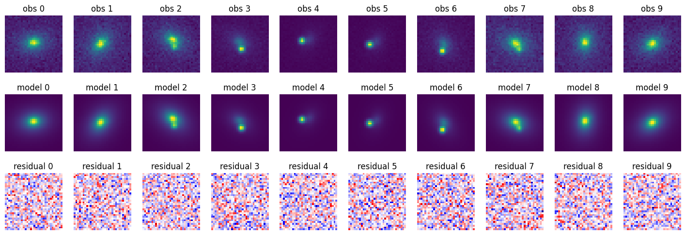
And to see the model in action we can sample it using the true parameter values. As expected, this produces a perfect set of residuals which look like pure random noise.
params_true = jnp.array(
    np.concatenate(
        [
            [0.7],  # sersic_q
            [np.pi / 4],  # sersic_PA
            [2.0],  # sersic_n
            [1.0],  # sersic_Re
            [1.0],  # sersic_Ie
            [0.4],  # sn_x
            [0.0],  # sn_y
            sn_flux(T),  # sn_flux
            np.array([0.1] * 10),  # sky
            np.array(dataset["crtan"].flatten()),  # crtan
        ]
    )
)
extra = (jnp.array(0.0), jnp.array(0.0), psf, dataset["crpix"], dataset["CD"])
sample = model(params_true, *extra)
residuals = (dataset["image"] - sample) / jnp.sqrt(dataset["variance"])
fig, axarr = plt.subplots(3, 10, figsize=(18, 6))
for i, (img, samp, resid) in enumerate(zip(dataset["image"], sample, residuals)):
    axarr[0, i].imshow(img.T, origin="lower", cmap="viridis")
    axarr[0, i].set_title(f"obs {i}")
    axarr[1, i].imshow(samp.T, origin="lower", cmap="viridis")
    axarr[1, i].set_title(f"model {i}")
    axarr[2, i].imshow(resid.T, origin="lower", cmap="seismic", vmin=-5, vmax=5)
    axarr[2, i].set_title(f"residual {i}")
for ax in axarr.flatten():
    ax.axis("off")
plt.show()
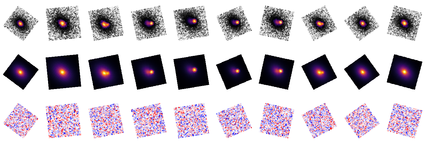
fig, axarr = plt.subplots(3, 10, figsize=(18, 6))
ap.plots.target_image(fig, axarr[0], apmodel.target)
ap.plots.model_image(fig, axarr[1], apmodel, showcbar=False)
ap.plots.residual_image(
    fig, axarr[2], apmodel, scaling="clip", normalize_residuals=True, showcbar=False
)
for ax in axarr.flatten():
    ax.axis("off")
plt.show()
# Let's compare how fast the two code are
print("Functional interface timings:")
%timeit jax.block_until_ready(model(params_true, *extra))
print("AstroPhot model timings:")
%timeit jax.block_until_ready(apmodel())
Functional interface timings:
6.31 ms ± 95.6 μs per loop (mean ± std. dev. of 7 runs, 100 loops each)
AstroPhot model timings:
221 ms ± 1.24 ms per loop (mean ± std. dev. of 7 runs, 1 loop each)
This is quite a striking result, the functional implementation is ~100x faster than the AstroPhot model! However, it is important to put this speed comparison in context. The AstroPhot model is much easier, less error prone, and more intuitive to put together. If we are only going to run the model a few times then we will save much more than 500ms by getting the code written faster. The cutout size of 32x32 is very small, while AstroPhot is built to scale to very large images. For larger images, the Python overhead is negligible and the two codes will have near identical runtime. In fact, if the images get a lot larger the functional version as written will run out of memory while the AstroPhot model could carry on easily because of how it chunks the data. Also, note that the plots are quite different, AstroPhot plots all the images properly oriented in the sky, while for the functional version we don’t have that capability. AstroPhot has a more complete understanding of the data and can perform a lot more operations on the results. AstroPhot could also combine in data at different resolutions and sizes, while our functional version is predicated on the idea that all the images will be 32x32 pixels, we would need to completely rewrite it to change that. If we wanted to change the model to fix some parameter or to turn one of the fixed parameters into a free parameter, we would have to trace it through the whole functional implementation and make updates accordingly. This goes for any change really, what if we needed to add in a mask, a second sersic model, or start modelling the PSF (rather than taking it as fixed); all of these would require painful changes to the functional version while they would be trivial additions to the AstroPhot model.
For these reasons and more, it is highly recommended to work with the object oriented AstroPhot models before ever considering the functional interface. And if you really need speed, jax.jit can get you 99.9% of the way there. Take a look at the timing comparison below, the AstroPhot model is now basically identical in speed to the laborious functional model:
jmodel = jax.jit(model)
_ = jax.block_until_ready(jmodel(params_true, *extra))
_ = jax.block_until_ready(jmodel(params_true, *extra))
print("JIT-compiled functional interface timings:")
%timeit jax.block_until_ready(jmodel(params_true, *extra))
japmodel = jax.jit(lambda: apmodel()._data)
_ = jax.block_until_ready(japmodel())
_ = jax.block_until_ready(japmodel())
print("JIT-compiled AstroPhot model timings:")
%timeit jax.block_until_ready(japmodel())
JIT-compiled functional interface timings:
5.5 ms ± 50.2 μs per loop (mean ± std. dev. of 7 runs, 100 loops each)
JIT-compiled AstroPhot model timings:
5.16 ms ± 8.67 μs per loop (mean ± std. dev. of 7 runs, 100 loops each)
# Make 8 chains, starting at the true parameters
params = np.stack(list(np.array(params_true) for _ in range(4)))

# Compute a mass matrix using the Fisher information matrix
J = jax.jacfwd(model, argnums=0)(params_true, *extra).reshape(-1, params_true.shape[-1])
V = dataset["variance"].reshape(-1)
H = J.T @ (J / V[:, None])
M = jnp.linalg.inv(H)


def log_likelihood(params, sersic_x, sersic_y, psf, crpix, CD):
    model_sample = model(params, sersic_x, sersic_y, psf, crpix, CD)
    residuals = (dataset["image"] - model_sample) ** 2 / dataset["variance"]
    return -0.5 * jnp.sum(residuals)


# Vectorized log likelihood and gradient functions
vmodel = jax.jit(jax.vmap(log_likelihood, in_axes=(0, None, None, None, None, None)))
vgmodel = jax.jit(
    jax.vmap(jax.grad(log_likelihood, argnums=0), in_axes=(0, None, None, None, None, None))
)

# Run MALA sampling
chain, logp = ap.fit.func.mala(
    params,
    lambda p: np.array(vmodel(jnp.array(p), *extra)),
    lambda p: np.array(vgmodel(jnp.array(p), *extra)),
    num_samples=400,
    epsilon=5e-1,
    mass_matrix=np.array(M),
)
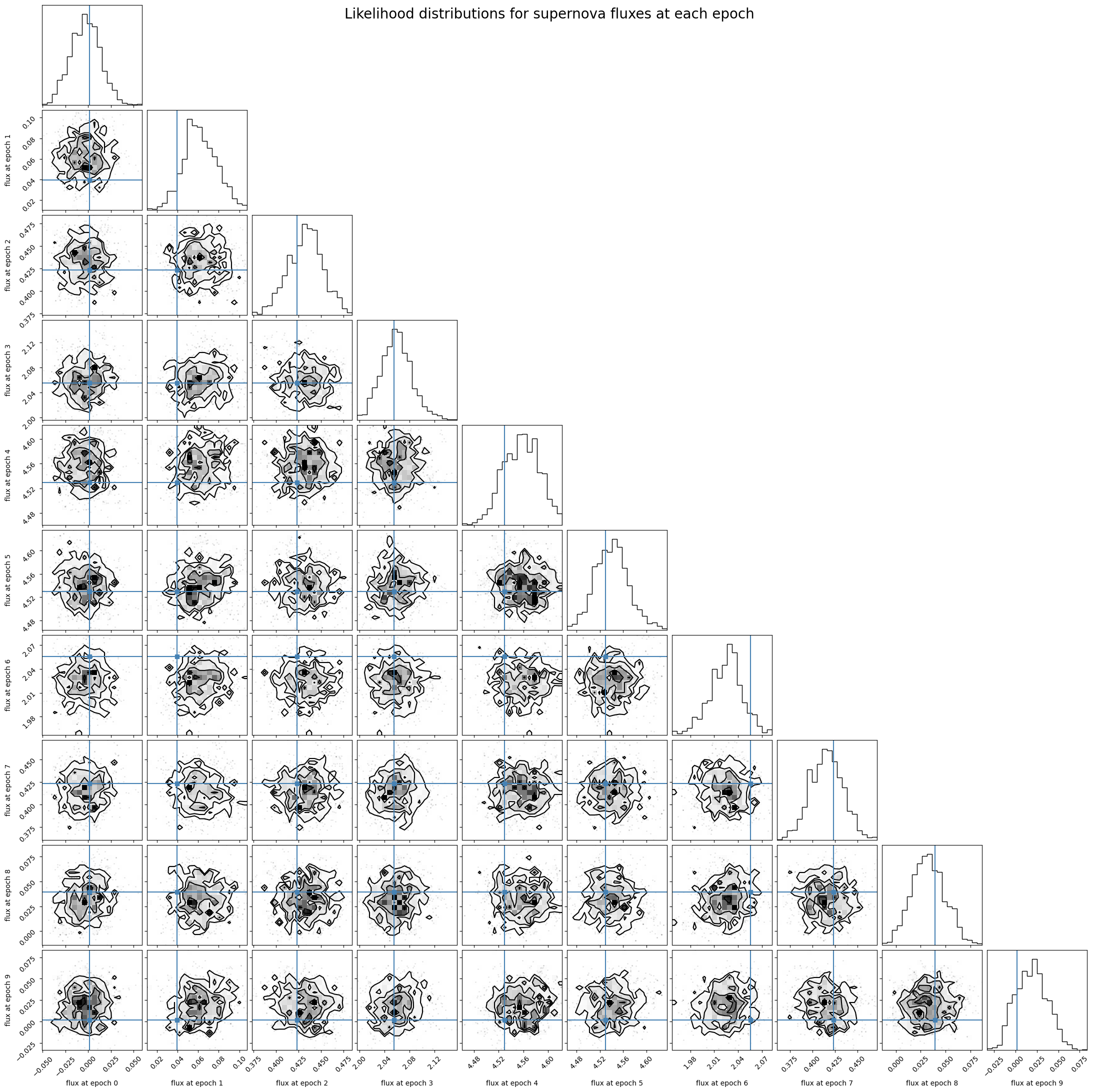
Now lets plot the likelihood distributions for the flux parameters compared to their true value. As you can see, the distributions do a good job of covering the ground truth! This means we have accurately extracted the light curve for the supernova data.
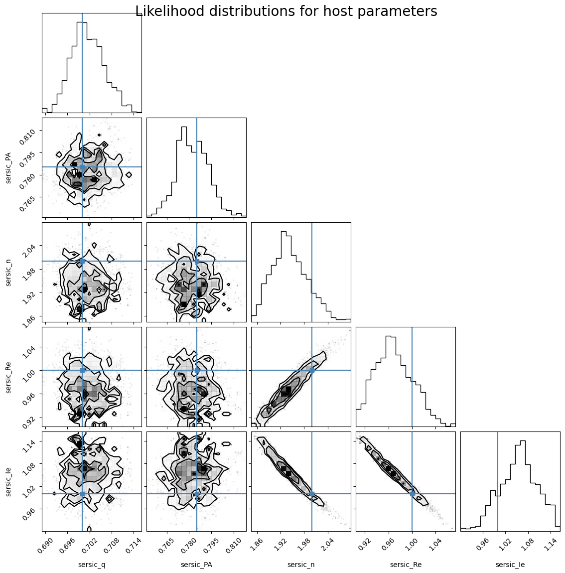
Below we show the likelihood distribution for the sersic host parameters. We can see that there is some non-linearity and certainly lots of correlation in these parameters. This makes the sampling a bit trickier, but MALA is up to the task.