Alternate Image Types

AstroPhot operates in the tangent plane space and so must have a mapping between the pixels and the sky that it can use to properly perform integration within every pixel. Aside from the standard ap.TargetImage used to store regular data with a linear mapping between pixel space and the tangent plane, there are two more image types ap.SIPTargetImage and ap.CMOSTargetImage which are explained below.

import astrophot as ap
import torch
import matplotlib.pyplot as plt
from matplotlib.patches import Rectangle
import numpy as np

SIP Target Image

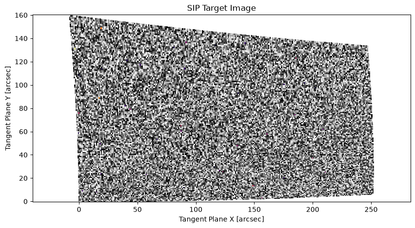
The ap.SIPTargetImage object stores data for a pixel array that is distorted using Simple-Image-Polynomial distortions. This is a non-linear polynomial transformation that is used to account for optical effects in images that result in the sky being non-linearly projected onto the pixel grid used to collect data. AstroPhot follows the WCS standard when it comes to SIP distortions and can read the SIP coefficients directly from an image. AstroPhot can also save a SIP distortion model to a FITS image. Internally the SIP coefficients are stored in image.sipA, image.sipB, image.sipAP and image.SIPBP which are formatted as dictionaries with the keys as tuples of two integers giving the powers and the value as the coefficient. For example in a FITS file the header line A_1_2 = 0.01 will translate to image.sipA = {(1,2): 0.01}.

Some particulars of the AstroPhot implementation. For the sake of efficiency, when a SIP image is created AstroPhot evaluates the SIP distortion at every pixel and stores that in a distortion map with the same size as the image. Afterwards, calling image.pixel_to_plane will not evaluate the SIP polynomial, but instead a bilinear interpolation of the distortion model will be used. This massively increases speed, but means that the distortion model is only accurate up to the bilinear interpolation accuracy, since most SIP distortions are quite smooth, this interpolation is extremely accurate. For queries beyond the borders of the image, AstroPhot will not extrapolate the SIP polynomials, instead the distortion amount at the pixel border is simply carried onwards. As second element of the AstroPhot implementation is that if a backwards model (AP and BP) is not provided, then AstroPhot will use linear algebra to determine the backwards model. This is taken from the very clever code written by Shu Liu and Lei Hi that you can find here.

For the most part, once you define a ap.SIPTargetImage you can use it like a regular ap.TargetImage object.

target = ap.SIPTargetImage(
    data=torch.randn(128, 256),
    sipA={(0, 1): 1e-3, (1, 0): -1e-3, (1, 1): 1e-4, (2, 0): -5e-5, (0, 2): -5e-4},
    sipB={(0, 1): 1e-3, (1, 0): -1e-3, (1, 1): -1e-3, (2, 0): 1e-4, (0, 2): 2e-3},
)

fig, ax = plt.subplots(figsize=(10, 5))
ap.plots.target_image(fig, ax, target)
ax.set_title("SIP Target Image")
plt.show()

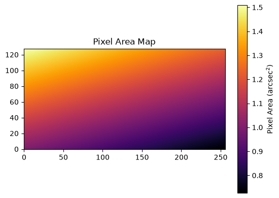
Because the pixels are distorted on the sky, this means that the amount of area on the sky for each pixel is different. One would expect a pixel that projects to a larger area to collect more light than one that gets squished smaller. A uniform source observed through a telescope with SIP distortions will therefore produce a non-uniform image. As such, AstroPhot tracks the projected area of each pixel to ensure its calculations are accurate. Here is what that pixel area map looks like for the above image. As you can see, the parts which get stretched out then correspond to larger areas, and the parts that get squished correspond to smaller areas.

plt.imshow(target.pixel_area_map.T, cmap="inferno", origin="lower")
plt.colorbar(label="Pixel Area (arcsec$^2$)")
plt.title("Pixel Area Map")
plt.show()

CMOS Target Image

A CMOS sensor is an alternative technology from a CCD for collecting light in an optical system. While it has certain advantages, one challenge with CMOS sensors is that only a sub region of each pixel is actually sensitive to light, the rest holding per-pixel electronics. This means there are gaps in the true placement of the CMOS pixels on the sky. Currently AstroPhot implements this by ensuring that the models are only sampled and integrated in the appropriate pixel areas. However, this treatment is not appropriate for certain PSF convolution modes and so the ap.CMOSTargetImage is under active development. Expect some changes in the future as we ensure it is viable for all model types. Currently, sky models, point source models, and un-convolved galaxy models should all work accurately. Adding convolved galaxy models is set for future work.

target = ap.CMOSTargetImage(
    data=torch.randn(128, 256),
    subpixel_loc=(-0.1, -0.1),
    subpixel_scale=0.8,
)

fig, ax = plt.subplots(figsize=(10, 5))
ap.plots.target_image(fig, ax, target)
ax.set_title("CMOS Target Image")
plt.show()

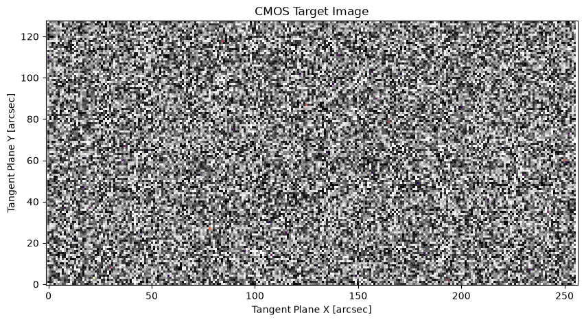
There is no visible difference when plotting the data as compressing every pixel in an image like above would make it hard to see what is happening. Below we plot what a single pixel truly looks like in the CMOS target representation.

fig, ax = plt.subplots(figsize=(5, 5))
r1 = Rectangle((-0.5, -0.5), 1, 1, facecolor="grey", label="Pixel Area")
ax.add_patch(r1)
r2 = Rectangle((-0.5, -0.5), 0.8, 0.8, facecolor="blue", label="Subpixel Area")
ax.add_patch(r2)
ax.scatter([-0.1], [-0.1], color="red", label="subpixel_loc")
ax.axvline(0.33, 0, 0.8, color="orange", linewidth=2, label="subpixel_scale")
ax.set_xlim(-0.5, 0.5)
ax.set_ylim(-0.5, 0.5)
ax.set_title("CMOS Pixel Representation")
ax.legend(loc="upper left")
plt.show()

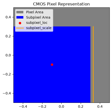
Where the blue subpixel area is actually sensitive to light. Note that pixel indexing places (0,0) at the center of the pixel and every pixel has size 1, so for the first pixel show here the pixel coordinates range from -0.5 to +0.5 on both axes. This is also the representation used to define a ap.CMOSTargetImage where subpixel_loc gives the pixel coordinates of the center of the subpixel and subpixel_scale gives the side length of the subpixel.

Batch Images

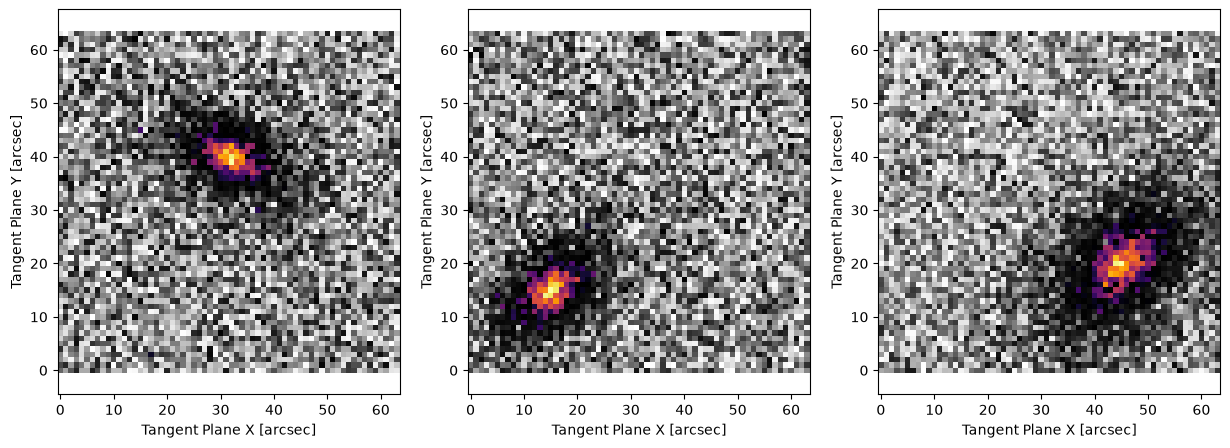
An ImageBatch is much like an ImageList except that it has certain restrictions applied to it. Namely that all the images must have the same size, and they must be of the “regular” image type, not SIP or CMOS. This extra constraint means they can’t be used as generally as other image types, but the trade off is extra computational advantages. You can see the batch scene model in the model zoo for one of the primary advantages of the ImageBatch image type. Another advantage is that it can be used to vectorize the fitting of images. Let’s say we have some simple model (either just a component model, or a full group model) and we want to use that same model to represent a bunch of similar images. We can use batched images to make this much more efficient. Rather than looping through the images one at a time, we can create a batch and set all their calculations to the hardware (CPU or GPU) at once. Here is an example of what this looks like, but the real advantage is when you seriously scale it up.

Note: Every dynamic parameter for the model must be batched, these are supposed to be independent models and so every parameter is unique for each model.

base_target = ap.TargetImage(data=np.zeros((64, 64)))
model = ap.Model(
    model_type="sersic galaxy model",
    name="batch_demo",
    center=(32, 40),
    q=0.6,
    PA=3.14 / 3,
    n=1,
    Re=10,
    Ie=1,
    target=base_target,
    integrate_mode="none",
    sampling_mode="quad:3",
)
model.initialize()

np.random.seed(42)
target1 = ap.TargetImage(
    name="target1", data=model().data + np.random.normal(scale=0.5, size=(64, 64))
)
model.center = (15, 15)
model.PA = -3.14 / 4
target2 = ap.TargetImage(
    name="target2", data=model().data + np.random.normal(scale=0.5, size=(64, 64))
)
model.center = (45, 20)
model.Re = 15
target3 = ap.TargetImage(
    name="target3", data=model().data + np.random.normal(scale=0.5, size=(64, 64))
)

batch_target = ap.TargetImageBatch([target1, target2, target3])
fig, axarr = plt.subplots(1, 3, figsize=(15, 5))
ap.plots.target_image(fig, axarr, batch_target)
plt.show()

# Every parameter must be batched
# Notice we set them a bit off the true values
model.center = ((30, 42), (16, 16), (46, 21))
model.q = (0.6, 0.6, 0.6)
model.PA = (3.14 / 3, -3.14 / 5, -3.14 / 4)
model.n = (1.1, 0.9, 1)
model.Re = (11, 11, 14)
model.Ie = (1, 0.8, 1.2)

res = ap.fit.BatchLM(model, batch_target, batch_target.window).fit()
print("Best-fit parameters:", res.current_state.detach().cpu().numpy())

fig, axarr = plt.subplots(2, 3, figsize=(15, 5))
for i in range(3):
    model.set_values(res.current_state[i])
    model.target = batch_target.images[i]
    ap.plots.model_image(fig, axarr[0, i], model)
    ap.plots.residual_image(fig, axarr[1, i], model)
plt.show()

==Starting LM fit for 'batch_demo' with batch of 3 images with 7 dynamic parameters and 4096 pixels==

Chi^2/DoF: [0.28872351 0.27383249 0.25914736], L: [1. 1. 1.]

/home/docs/checkouts/readthedocs.org/user_builds/astrophot/envs/stable/lib/python3.12/site-packages/torch/jit/_script.py:1488: DeprecationWarning: `torch.jit.script` is deprecated. Please switch to `torch.compile` or `torch.export`.
  warnings.warn(

Chi^2/DoF: [0.25300431 0.26015994 0.24308725], L: [0.00137174 0.13580247 0.00137174]

Chi^2/DoF: [0.24882743 0.25932468 0.24256457], L: [1.86285966e-04 1.86285966e-04 1.88167642e-06]

Chi^2/DoF: [0.24863835 0.25928234 0.24256112], L: [2.55536304e-07 2.55536304e-07 2.58117479e-09]

Final Chi^2/DoF: [0.2486377  0.25928215 0.24256112], L: [3.47024611e-08 9.99999972e-10 3.47024611e-08]. Converged: success

Best-fit parameters: [[32.00015604 39.90013343  0.59057318  1.08720111  1.09507162 10.46204472
   0.91542374]
 [15.10946574 15.0098841   0.60067376  2.30124813  0.90120912  9.19815529
   1.13302337]
 [45.18876438 19.85669346  0.60387853  2.37013704  1.0143141  14.86376428
   0.99759275]]

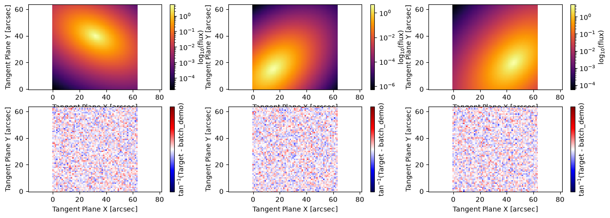
And there we have it! Three models fit at once. Really, just doing three isn’t a big deal computationally. But if you have dozens or hundreds of these little 64x64 pixel images then grouping them all together can get huge computational speedups. If you are able to run these big batched fits on a GPU you can get several orders of magnitude runtime reduction!

Happy fitting!