Joint Modelling

In this tutorial you will learn how to set up a joint modelling fit which encoporates the data from multiple images. These use GroupModel objects just like in the GroupModels.ipynb tutorial, the main difference being how the TargetImage object is constructed and that more care must be taken when assigning targets to models.

It is, of course, more work to set up a fit across multiple target images. However, the tradeoff can be well worth it. Perhaps there is space-based data with high resolution, but groundbased data has better S/N. Or perhaps each band individually does not have enough signal for a confident fit, but all three together just might. Perhaps colour information is of paramount importance for a science goal, one would hope that both bands could be treated on equal footing but in a consistent way when extracting profile information. There are a number of reasons why one might wish to try and fit a multi image picture of a galaxy simultaneously.

When fitting multiple bands one often resorts to forced photometry, sometimes also blurring each image to the same approximate PSF. With AstroPhot this is entirely unnecessary as one can fit each image in its native PSF simultaneously. The final fits are more meaningful and can encorporate all of the available structure information.

import astrophot as ap
import matplotlib.pyplot as plt
from astropy.io import fits

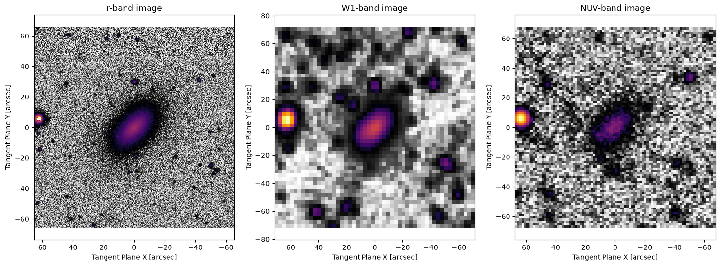
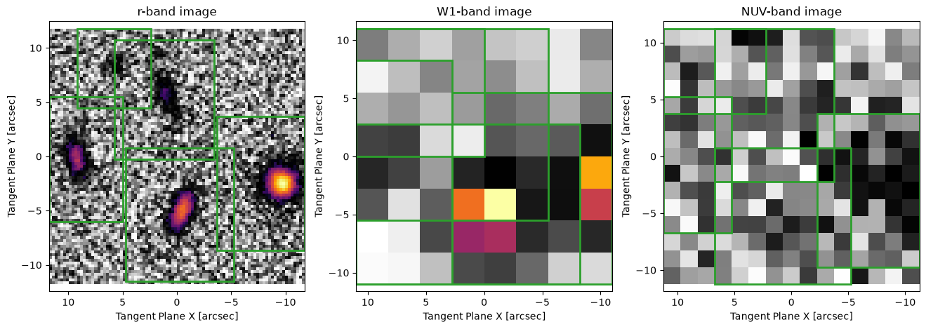
# First we need some data to work with, let's use LEDA 41136 as our example galaxy

# The images must be aligned to a common coordinate system. From the DESI Legacy survey we are extracting
# each image using its RA and DEC coordinates, the WCS in the FITS header will ensure a common coordinate system.

# It is also important to have a good estimate of the variance and the PSF for each image since these
# affect the relative weight of each image. For the tutorial we use simple approximations, but in
# science level analysis one should endeavor to get the best measure available for these.

############ UNCOMMENT IF RUNNING LOCALLY ############
# hdu = fits.open(
#     "https://www.legacysurvey.org/viewer/fits-cutout?ra=187.3119&dec=12.9783&size=500&layer=ls-dr9&pixscale=0.262&bands=r"
# )
# hdu.writeto("joint_target_image_r.fits", overwrite=True)
# hdu = fits.open(
#     "https://www.legacysurvey.org/viewer/fits-cutout?ra=187.3119&dec=12.9783&size=52&layer=unwise-neo7&pixscale=2.75&bands=1"
# )
# hdu.writeto("joint_target_image_W1.fits", overwrite=True)
# hdu = fits.open(
#     "https://www.legacysurvey.org/viewer/fits-cutout?ra=187.3119&dec=12.9783&size=90&layer=galex&pixscale=1.5&bands=n"
# )
# hdu.writeto("joint_target_image_NUV.fits", overwrite=True)

# Our first image is from the DESI Legacy-Survey r-band. This image has a pixelscale of 0.262 arcsec/pixel and is 500 pixels across
target_r = ap.TargetImage(
    filename="joint_target_image_r.fits",
    zeropoint=22.5,
    variance="auto",  # auto variance gets it roughly right, use better estimate for science!
    psf=ap.utils.initialize.gaussian_psf(1.12 / 2.355, 51, 0.262),
    name="rband",
)


# The second image is a unWISE W1 band image. This image has a pixelscale of 2.75 arcsec/pixel and is 52 pixels across
target_W1 = ap.TargetImage(
    filename="joint_target_image_W1.fits",
    zeropoint=25.199,
    variance="auto",
    psf=ap.utils.initialize.gaussian_psf(6.1 / 2.355, 21, 2.75),
    name="W1band",
)

# The third image is a GALEX NUV band image. This image has a pixelscale of 1.5 arcsec/pixel and is 90 pixels across
target_NUV = ap.TargetImage(
    filename="joint_target_image_NUV.fits",
    zeropoint=20.08,
    variance="auto",
    psf=ap.utils.initialize.gaussian_psf(5.4 / 2.355, 21, 1.5),
    name="NUVband",
)

fig1, ax1 = plt.subplots(1, 3, figsize=(18, 6))
ap.plots.target_image(fig1, ax1[0], target_r)
ax1[0].set_title("r-band image")
ap.plots.target_image(fig1, ax1[1], target_W1)
ax1[1].set_title("W1-band image")
ap.plots.target_image(fig1, ax1[2], target_NUV)
ax1[2].set_title("NUV-band image")
plt.show()

# The joint model will need a target to try and fit, but now that we have multiple images the "target" is
# a Target_Image_List object which points to all three.
target_full = ap.TargetImageList((target_r, target_W1, target_NUV))
# It doesn't really need any other information since everything is already available in the individual targets

# To make things easy to start, lets just fit a sersic model to all three. In principle one can use arbitrary
# group models designed for each band individually, but that would be unnecessarily complex for a tutorial

model_r = ap.Model(
    name="rband_model",
    model_type="sersic galaxy model",
    target=target_r,
    psf_convolve=True,
)

model_W1 = ap.Model(
    name="W1band_model",
    model_type="sersic galaxy model",
    target=target_W1,
    center=[0, 0],
    PA=-2.3,
    psf_convolve=True,
)

model_NUV = ap.Model(
    name="NUVband_model",
    model_type="sersic galaxy model",
    target=target_NUV,
    center=[0, 0],
    PA=-2.3,
    psf_convolve=True,
)

# At this point we would just be fitting three separate models at the same time, not very interesting. Next
# we add constraints so that some parameters are shared between all the models. It makes sense to fix
# structure parameters while letting brightness parameters vary between bands so that's what we do here.
for p in ["center", "q", "PA", "n", "Re"]:
    model_W1[p].value = model_r[p]
    model_NUV[p].value = model_r[p]
# Now every model will have a unique Ie, but every other parameter is shared

# We can now make the joint model object

model_full = ap.Model(
    name="LEDA41136",
    model_type="group model",
    models=[model_r, model_W1, model_NUV],
    target=target_full,
)

model_full.initialize()
model_full.graphviz()

Initializing model rband_model

Initializing model W1band_model

Initializing model NUVband_model

result = ap.fit.LM(model_full, verbose=1).fit()
print(result.message)

==Starting LM fit for 'LEDA41136' with 9 dynamic parameters and 260804 pixels==

Chi^2/DoF: 13.4329, L: 1

/home/docs/checkouts/readthedocs.org/user_builds/astrophot/envs/stable/lib/python3.12/site-packages/torch/jit/_script.py:1488: DeprecationWarning: `torch.jit.script` is deprecated. Please switch to `torch.compile` or `torch.export`.
  warnings.warn(

Chi^2/DoF: 13.0319, L: 0.111

Chi^2/DoF: 12.8803, L: 1.22

Chi^2/DoF: 12.843, L: 1.22

Chi^2/DoF: 12.7649, L: 0.136

Chi^2/DoF: 12.7219, L: 0.0151

Chi^2/DoF: 12.7207, L: 0.000186

Final Chi^2/DoF: 12.7207, L: 0.000186. Converged: success

success

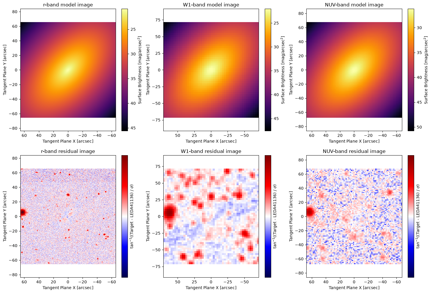
# here we plot the results of the fitting, notice that each band has a different PSF and pixelscale. Also, notice
# that the colour bars represent significantly different ranges since each model was allowed to fit its own Ie.
# meanwhile the center, PA, q, and Re is the same for every model.
fig1, ax1 = plt.subplots(2, 3, figsize=(18, 12))
ap.plots.model_image(fig1, ax1[0], model_full)
ax1[0][0].set_title("r-band model image")
ax1[0][1].set_title("W1-band model image")
ax1[0][2].set_title("NUV-band model image")
ap.plots.residual_image(fig1, ax1[1], model_full, normalize_residuals=True)
ax1[1][0].set_title("r-band residual image")
ax1[1][1].set_title("W1-band residual image")
ax1[1][2].set_title("NUV-band residual image")
plt.show()

Joint models with multiple models

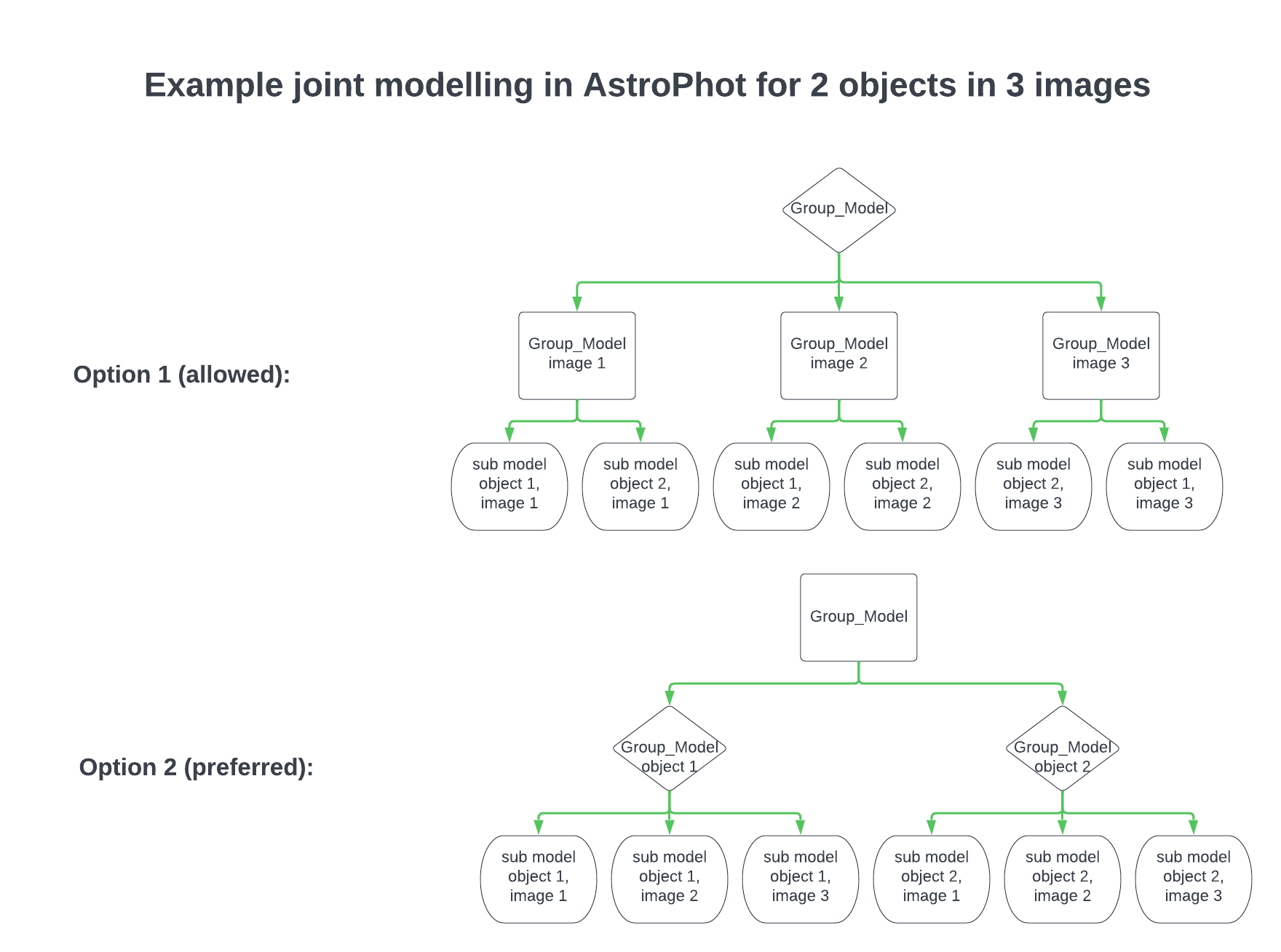
If you want to analyze more than a single astronomical object, you will need to combine many models for each image in a reasonable structure. There are a number of ways to do this that will work, though may not be as scalable. For small images, just about any arrangement is fine when using the LM optimizer. But as images and number of models scales very large, it may be necessary to sub divide the problem to save memory. To do this you should arrange your models in a hierarchy so that AstroPhot has some information about the structure of your problem. There are two ways to do this. First, you can create a group of models where each sub-model is a group which holds all the objects for one image. Second, you can create a group of models where each sub-model is a group which holds all the representations of a single astronomical object across each image. The second method is preferred. See the diagram below to help clarify what this means.

JointGroupModels

Here we will see an example of a multiband fit of an image which has multiple astronomical objects.

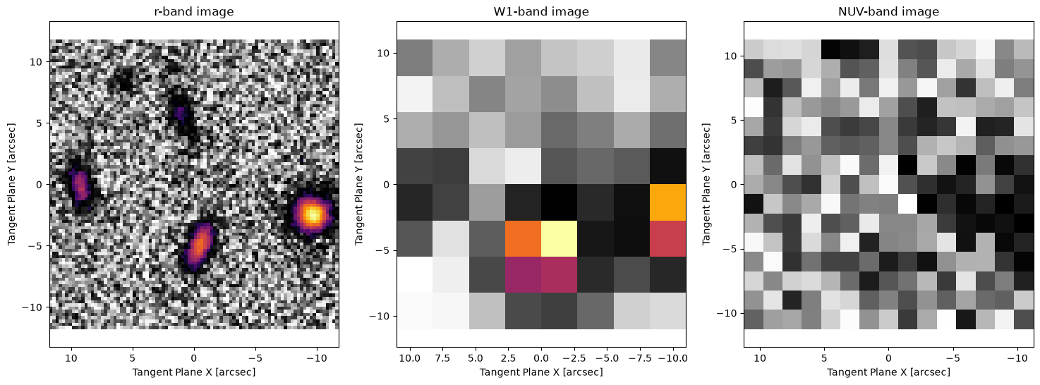
# First we need some data to work with, let's use another LEDA object, this time a group of galaxies: LEDA 389779, 389797, 389681

RA = 156.7283
DEC = 15.5512
# Our first image is from the DESI Legacy-Survey r-band. This image has a pixelscale of 0.262 arcsec/pixel
rsize = 90
wsize = int(rsize * 0.262 / 2.75)
gsize = int(rsize * 0.262 / 1.5)

# Now we make our targets
############ UNCOMMENT IF RUNNING LOCALLY ############
# hdu = fits.open(
#     f"https://www.legacysurvey.org/viewer/fits-cutout?ra={RA}&dec={DEC}&size={rsize}&layer=ls-dr9&pixscale=0.262&bands=r"
# )
# hdu.writeto("joint_group_target_image_r.fits", overwrite=True)
# hdu = fits.open(
#     f"https://www.legacysurvey.org/viewer/fits-cutout?ra={RA}&dec={DEC}&size={wsize}&layer=unwise-neo7&pixscale=2.75&bands=1"
# )
# hdu.writeto("joint_group_target_image_W1.fits", overwrite=True)
# hdu = fits.open(
#     f"https://www.legacysurvey.org/viewer/fits-cutout?ra={RA}&dec={DEC}&size={gsize}&layer=galex&pixscale=1.5&bands=n"
# )
# hdu.writeto("joint_group_target_image_NUV.fits", overwrite=True)
target_r = ap.image.TargetImage(
    filename="joint_group_target_image_r.fits",
    zeropoint=22.5,
    variance="auto",
    psf=ap.utils.initialize.gaussian_psf(1.12 / 2.355, 51, 0.262),
    name="rband",
)

# The second image is a unWISE W1 band image. This image has a pixelscale of 2.75 arcsec/pixel
target_W1 = ap.image.TargetImage(
    filename="joint_group_target_image_W1.fits",
    zeropoint=25.199,
    variance="auto",
    psf=ap.utils.initialize.gaussian_psf(6.1 / 2.355, 21, 2.75),
    name="W1band",
)

# The third image is a GALEX NUV band image. This image has a pixelscale of 1.5 arcsec/pixel
target_NUV = ap.image.TargetImage(
    filename="joint_group_target_image_NUV.fits",
    zeropoint=20.08,
    variance="auto",
    psf=ap.utils.initialize.gaussian_psf(5.4 / 2.355, 21, 1.5),
    name="NUVband",
)
target_full = ap.image.TargetImageList((target_r, target_W1, target_NUV))

fig1, ax1 = plt.subplots(1, 3, figsize=(18, 6))
ap.plots.target_image(fig1, ax1, target_full)
ax1[0].set_title("r-band image")
ax1[1].set_title("W1-band image")
ax1[2].set_title("NUV-band image")
plt.show()

#########################################
# NOTE: photutils is not a dependency of AstroPhot, make sure you run: pip install photutils
# if you dont already have that package. Also note that you can use any segmentation map
# code, we just use photutils here because it is very easy.
#########################################
from photutils.segmentation import detect_sources, deblend_sources

rdata = target_r.data.detach().cpu().numpy()
initsegmap = detect_sources(rdata, threshold=0.01, npixels=10)
segmap = deblend_sources(rdata, initsegmap, npixels=5).data
fig8, ax8 = plt.subplots(figsize=(8, 8))
ax8.imshow(segmap, origin="lower", cmap="inferno")
plt.show()
# This will convert the segmentation map into boxes that enclose the identified pixels
rwindows = ap.utils.initialize.windows_from_segmentation_map(segmap)
# Next we scale up the windows so that AstroPhot can fit the faint parts of each object as well
rwindows = ap.utils.initialize.scale_windows(
    rwindows, image=target_r, expand_scale=1.5, expand_border=10
)
w1windows = ap.utils.initialize.transfer_windows(rwindows, target_r, target_W1)
w1windows = ap.utils.initialize.scale_windows(w1windows, image=target_W1, expand_border=1)
nuvwindows = ap.utils.initialize.transfer_windows(rwindows, target_r, target_NUV)
# Here we get some basic starting parameters for the galaxies (center, position angle, axis ratio)
centers = ap.utils.initialize.centroids_from_segmentation_map(segmap, target_r)
PAs = ap.utils.initialize.PA_from_segmentation_map(segmap, target_r, centers)
qs = ap.utils.initialize.q_from_segmentation_map(segmap, target_r, centers)

There is barely any signal in the GALEX data and it would be entirely impossible to analyze on its own. With simultaneous multiband fitting it is a breeze to get relatively robust results!

Next we need to construct models for each galaxy. This is understandably more complex than in the single band case, since now we have three times the amount of data to keep track of. Recall that we will create a number of joint models to represent each astronomical object, then put them all together in a larger group model.

model_list = []

for i, window in enumerate(rwindows):
    # create the submodels for this object
    sub_list = []
    sub_list.append(
        ap.Model(
            name=f"rband_model_{i}",
            model_type="sersic galaxy model",  # we could use spline models for the r-band since it is well resolved
            target=target_r,
            window=rwindows[window],
            psf_convolve=True,
            center=centers[window],
            PA=PAs[window],
            q=qs[window],
        )
    )
    sub_list.append(
        ap.Model(
            name=f"W1band_model_{i}",
            model_type="sersic galaxy model",
            target=target_W1,
            window=w1windows[window],
            psf_convolve=True,
        )
    )
    sub_list.append(
        ap.Model(
            name=f"NUVband_model_{i}",
            model_type="sersic galaxy model",
            target=target_NUV,
            window=nuvwindows[window],
            psf_convolve=True,
        )
    )
    # ensure equality constraints
    # across all bands, same center, q, PA, n, Re
    for p in ["center", "q", "PA", "n", "Re"]:
        sub_list[1][p].value = sub_list[0][p]
        sub_list[2][p].value = sub_list[0][p]

    # Make the multiband model for this object
    model_list.append(
        ap.Model(
            name=f"model_{i}",
            model_type="group model",
            target=target_full,
            models=sub_list,
        )
    )
# Make the full model for this system of objects
MODEL = ap.Model(
    name=f"full_model",
    model_type="group model",
    target=target_full,
    models=model_list,
)
fig, ax = plt.subplots(1, 3, figsize=(16, 5))
ap.plots.target_image(fig, ax, MODEL.target)
ap.plots.model_window(fig, ax, MODEL)
ax[0].set_title("r-band image")
ax[1].set_title("W1-band image")
ax[2].set_title("NUV-band image")
plt.show()

MODEL.initialize()
MODEL.graphviz()

Initializing model model_0

Initializing model rband_model_0

Initializing model W1band_model_0

Initializing model NUVband_model_0

Initializing model model_1

Initializing model rband_model_1

Initializing model W1band_model_1

Initializing model NUVband_model_1

Initializing model model_2

Initializing model rband_model_2

Initializing model W1band_model_2

Initializing model NUVband_model_2

Initializing model model_3

Initializing model rband_model_3

Initializing model W1band_model_3

Initializing model NUVband_model_3

Initializing model model_4

Initializing model rband_model_4

Initializing model W1band_model_4

Initializing model NUVband_model_4

# We give it only one iteration for runtime/demo purposes, you should let these algorithms run to convergence
result = ap.fit.Iter(MODEL, verbose=1, max_iter=1).fit()

--------iter-------

model_0

model_1

model_2

model_3

model_4

Update Chi^2 with new parameters

Loss: 2.327178059016913

fig1, ax1 = plt.subplots(2, 3, figsize=(18, 11))
ap.plots.model_image(fig1, ax1[0], MODEL, vmax=30)
ax1[0][0].set_title("r-band model image")
ax1[0][1].set_title("W1-band model image")
ax1[0][2].set_title("NUV-band model image")
ap.plots.residual_image(fig1, ax1[1], MODEL, normalize_residuals=True)
ax1[1][0].set_title("r-band residual image")
ax1[1][1].set_title("W1-band residual image")
ax1[1][2].set_title("NUV-band residual image")
plt.show()

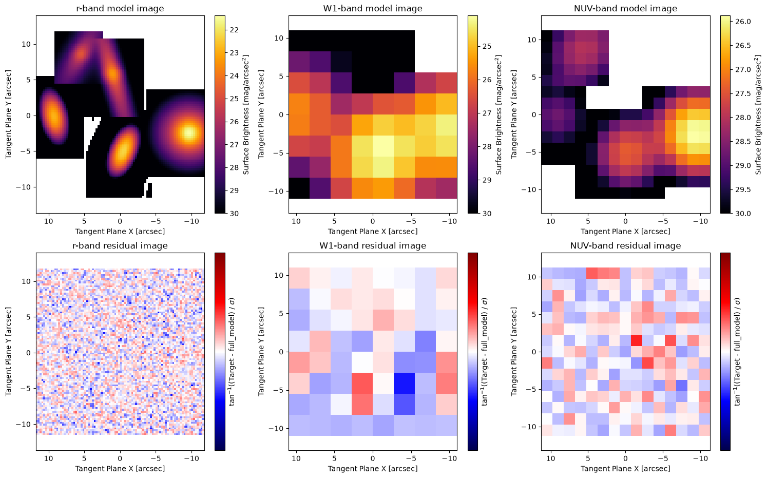
The models look pretty good! The power of multiband fitting lets us know that we have extracted all the available information here, no forced photometry required! Some notes though, since we didn’t fit a sky model, the colourbars are quite extreme.

An important note here is that the SB levels for the W1 and NUV data are quire reasonable. While the structure (center, PA, q, n, Re) was shared between bands and therefore mostly driven by the r-band, the brightness is entirely independent between bands meaning the Ie (and therefore SB) values are right from the W1 and NUV data!

These residuals mostly look like just noise! The only feature remaining is the row on the bottom of the W1 image. This could likely be fixed by running the fit to convergence and/or taking a larger FOV.

Dithered images

Note that it is not necessary to use images from different bands. Using dithered images one can effectively achieve higher resolution. It is possible to simultaneously fit dithered images with AstroPhot instead of postprocessing the two images together. This will of course be slower, but may be worthwhile for cases where extra care is needed.

Stacked images

Like dithered images, one may wish to combine the statistical power of multiple images but for some reason it is not clear how to add them (for example they are at different rotations). In this case one can simply have AstroPhot fit the images simultaneously. Again this is slower than if the image could be combined, but should extract all the statistical power from the data!

Time series

Some objects change over time. For example they may get brighter and dimmer, or may have a transient feature appear. However, the structure of an object may remain constant. An example of this is a supernova and its host galaxy. The host galaxy likely doesn’t change across images, but the supernova does. It is possible to fit a time series dataset with a shared galaxy model across multiple images, and a shared position for the supernova, but a variable brightness for the supernova over each image.

It is possible to get quite creative with joint models as they allow one to fix selective features of a model over a wide range of data. If you have a situation which may benefit from joint modelling but are having a hard time determining how to format everything, please do contact us!