Model Zoo

In this notebook you will see every kind of model in AstroPhot. Printed in each cell will also be the list of parameters which the model looks for while fitting. Many models have unique capabilities and features, this will be introduced here, though fully taking advantage of them will be dependent on your science case.

Note, we will not be covering GroupModel here as that requires a dedicated discussion. See the dedicated notebook for that.

%load_ext autoreload
%autoreload 2
%matplotlib inline

import astrophot as ap
import numpy as np
import matplotlib.pyplot as plt
import matplotlib.animation as animation
from IPython.display import HTML

basic_target = ap.TargetImage(data=np.zeros((100, 100)), pixelscale=1, zeropoint=20)

Sky Models

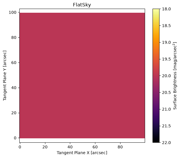
Flat Sky Model

M = ap.Model(model_type="flat sky model", center=[50, 50], I0=1, target=basic_target)
M.initialize()

fig, ax = plt.subplots(figsize=(7, 6))
ap.plots.model_image(fig, ax, M)
ax.set_title(M.name)
plt.show()

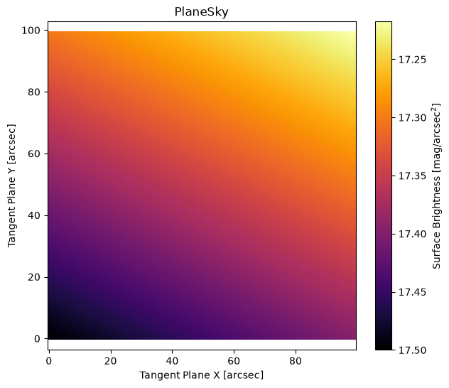
Plane Sky Model

M = ap.Model(
    model_type="plane sky model",
    center=[50, 50],
    I0=10,
    delta=[1e-2, 2e-2],
    target=basic_target,
)
M.initialize()

fig, ax = plt.subplots(figsize=(7, 6))
ap.plots.model_image(fig, ax, M)
ax.set_title(M.name)
plt.show()

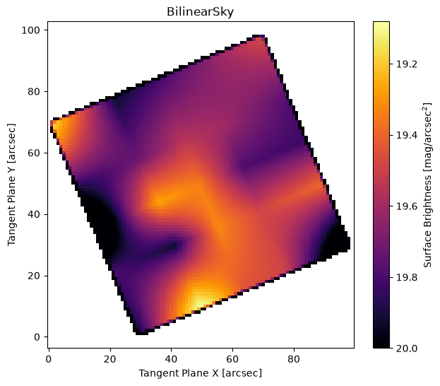
Bilinear Sky Model

This allows for a complex sky model which can vary arbitrarily as a function of position. Here we plot a sky that is just noise, but one would typically make it smoothly varying. The noise sky makes the nature of bilinear interpolation very clear, large flux changes can create sharp edges in the reconstruction.

Here we show how you can set the PA and scale manually, if you don’t provide those arguments they will automatically be set to fill the target image (which is usually what you want).

np.random.seed(42)
M = ap.Model(
    model_type="bilinear sky model",
    I=np.random.uniform(0, 1, (5, 5)) + 1,
    PA=np.pi / 8,
    scale=15,
    target=basic_target,
)
M.initialize()

fig, ax = plt.subplots(figsize=(7, 6))
ap.plots.model_image(fig, ax, M, vmax=20)
ax.set_title(M.name)
plt.show()

Point Source Function (PSF) Models

These models are well suited to describe stars or any other point like source of light, they may also be used to convolve with other models during optimization. Some things to keep in mind about PSF models:

• Their “target” should be a PSFImage object

• They are always centered at (0,0) so there is no need to optimize the center position

• Their total flux is typically normalized to 1, so no need to optimize any normalization parameters

• They can be used in a lot of places that a PSFImage can be used, such as the convolution kernel for a model

They behave a bit differently than other models, see the point source model further down. A PSF describes the abstract point source light distribution, to actually model a star in a field you will need a point model object (further down) to represent a delta function of brightness with some total flux.

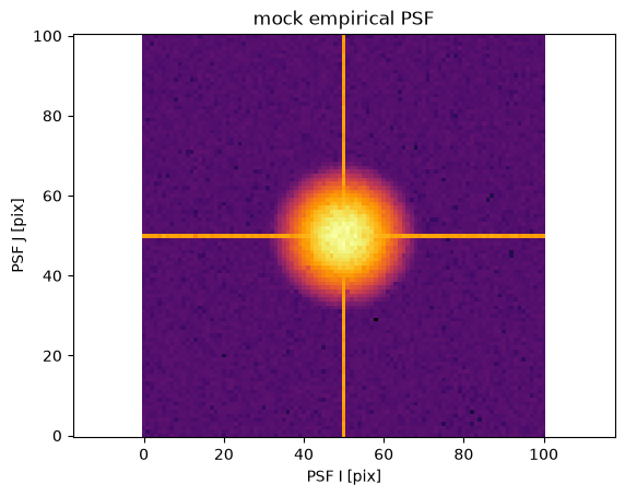
np.random.seed(124)
psf = ap.utils.initialize.gaussian_psf(3.0, 101, 1.0)
psf[50] += np.mean(psf)
psf[:, 50] += np.mean(psf)
psf += 1e-10
psf += np.random.normal(scale=psf / 3)
psf[psf < 0] = ap.utils.initialize.gaussian_psf(3.0, 101, 1.0)[psf < 0] + 1e-10

psf_target = ap.PSFImage(
    data=psf / np.sum(psf),
    upsample=1,
)
fig, ax = plt.subplots()
ap.plots.psf_image(fig, ax, psf_target)
ax.set_title("mock empirical PSF")
plt.show()

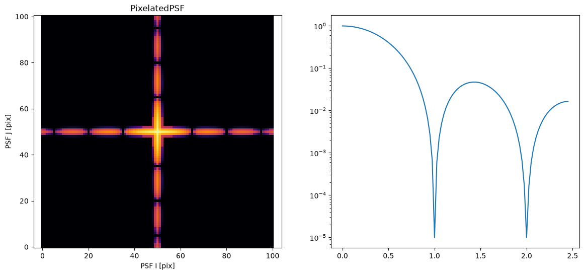
Pixelated point source

Note that in this model you can define an arbitrary pixel map, for the sake of demonstration we build an extremely oversimplified mock diffraction spike model.

from scipy.special import sinc

xx, yy = np.meshgrid(np.linspace(-50, 50, 101), np.linspace(-50, 50, 101))
x = np.sqrt(xx**2 + yy**2) / 15
PSF = np.zeros_like(x) + 1e-6
wgt = np.array((0.0001, 0.01, 1.0, 0.01, 0.0001))
PSF[48:53] += (sinc(x[48:53]) ** 2) * wgt.reshape((-1, 1))
PSF[:, 48:53] += (sinc(x[:, 48:53]) ** 2) * wgt
PSF = ap.PSFImage(data=PSF)

M = ap.Model(
    model_type="pixelated psf model",
    target=psf_target,
    pixels=PSF.data / psf_target.pixel_area,
)
M.initialize()

fig, ax = plt.subplots(1, 2, figsize=(14, 6))
ap.plots.psf_image(fig, ax[0], M)
x = np.linspace(0, 49, 99) / 20
ax[1].plot(x, sinc(x) ** 2 + 1e-5)
ax[1].set_yscale("log")
ax[0].set_title(M.name)
plt.show()

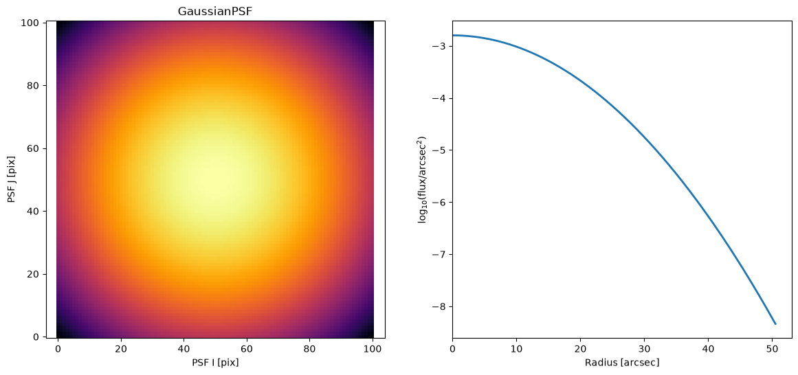
Gaussian PSF

Never a great PSF model, but the Gaussian is simple. This makes it a good starting choice to get results before stepping up the complexity level.

M = ap.Model(model_type="gaussian psf model", sigma=10, target=psf_target)
M.initialize()
fig, ax = plt.subplots(1, 2, figsize=(14, 6))
ap.plots.psf_image(fig, ax[0], M)
ap.plots.radial_light_profile(fig, ax[1], M)
ax[0].set_title(M.name)
plt.show()

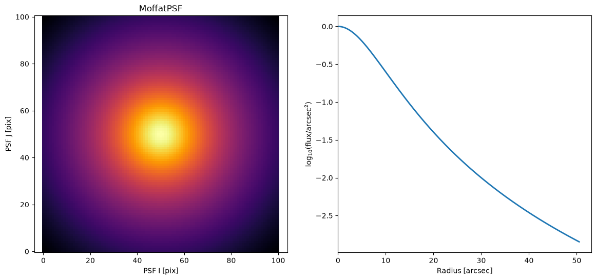
Moffat PSF

A circular PSF model using a Moffat light profile

Note: All of the radial profiles for GalaxyModel types (sersic, ferrer, exponential, moffat, king, spline, gaussian, nuker) are available for PSFModel’s (including an ellipse counterpart).

M = ap.Model(model_type="moffat psf model", n=2.0, Rd=10.0, target=psf_target)
M.initialize()

fig, ax = plt.subplots(1, 2, figsize=(14, 6))
ap.plots.psf_image(fig, ax[0], M)
ap.plots.radial_light_profile(fig, ax[1], M)
ax[0].set_title(M.name)
plt.show()

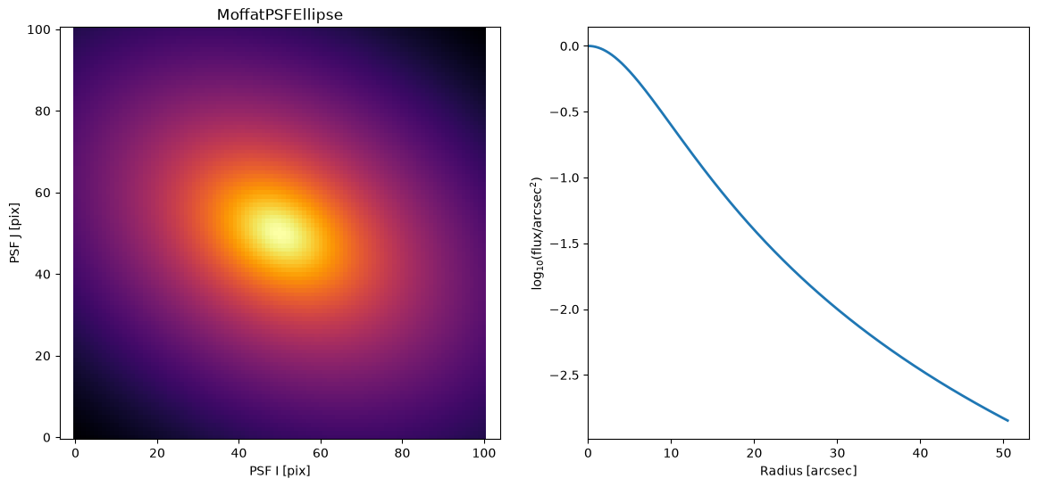
2D Moffat PSF

Like a Moffat, but can have a axis ratio and position angle. This could be used to make parametric spikes, or account for very slight asymmetry in a PSF.

M = ap.Model(
    model_type="moffat ellipse psf model",
    n=2.0,
    Rd=10.0,
    q=0.7,
    PA=3.14 / 3,
    target=psf_target,
)
M.initialize()

fig, ax = plt.subplots(1, 2, figsize=(14, 6))
ap.plots.psf_image(fig, ax[0], M)
ap.plots.radial_light_profile(fig, ax[1], M)
ax[0].set_title(M.name)
plt.show()

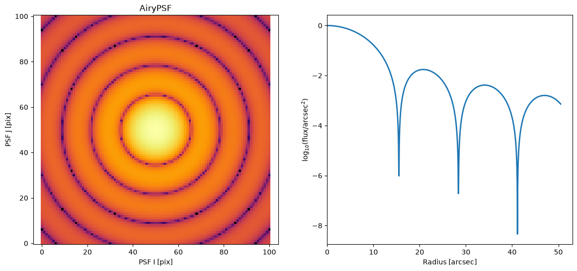
Airy disk PSF

M = ap.Model(
    model_type="airy psf model",
    R1=15.5,
    target=psf_target,
)
M.initialize()

fig, ax = plt.subplots(1, 2, figsize=(14, 6))
ap.plots.psf_image(fig, ax[0], M)
ap.plots.radial_light_profile(fig, ax[1], M)
ax[0].set_title(M.name)
plt.show()

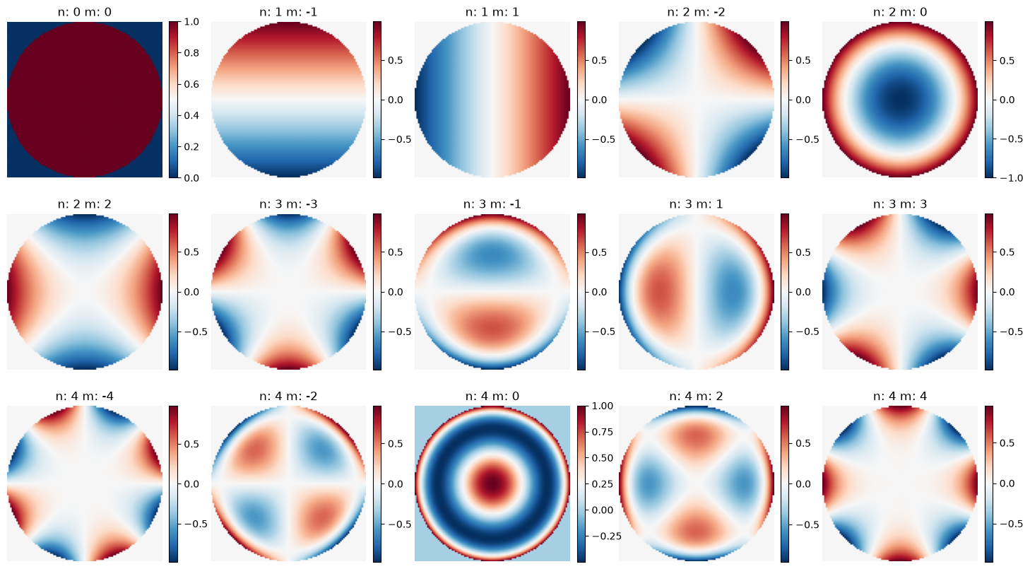
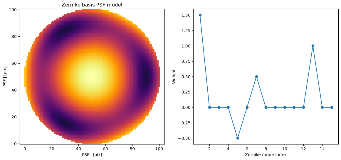
Basis PSF

A basis psf model allows one to provide a series of images such as an Eigen decomposition or a Zernike polynomial (or any other basis one likes). The weight of each component is fit to determine the final model. If a suitable basis is chosen then it is possible to encode highly complex models with only a few free parameters as the weights.

For the basis argument one may provide the basis manually (N imgs, H, W) or simply provide "zernike:n" where n gives the Zernike order up to which will be fit.

As the basis may be provided manually, one can even provide a base PSF model as the first component and then use the Zernike coefficients as perturbations.

w = [1.5, 0, 0, 0.0, -0.5, 0, 0.5, 0, 0, 0, 0.0, 0, 1, 0, 0]
M = ap.Model(model_type="basis psf model", basis="zernike:4", weights=w, target=psf_target)
M.initialize()
nm_list = ap.models.func.zernike_n_m_list(4)
fig, axarr = plt.subplots(3, 5, figsize=(18, 10))
for i, ax in enumerate(axarr.flatten()):
    ax.set_title(f"n: {nm_list[i][0]} m: {nm_list[i][1]}")
    ax.imshow(M.basis[i], cmap="RdBu_r", origin="lower")
    plt.colorbar(ax.images[0], ax=ax, fraction=0.046, pad=0.04)
    ax.axis("off")
plt.show()
fig, ax = plt.subplots(1, 2, figsize=(14, 6))
ap.plots.psf_image(fig, ax[0], M, vmin=5e-5)
ax[1].plot(np.arange(1, 16), M.weights.value.numpy(), marker="o")
ax[1].set_xlabel("Zernike mode index")
ax[1].set_ylabel("Weight")
ax[0].set_title("Zernike basis PSF model")
plt.show()

The Point Source Model

This model is used to represent point sources in the sky such as stars, supernovae, asteroids, small galaxies, quasars, and more. It is effectively a delta function at a given position with a given flux. Otherwise it has no structure. You must provide it a PSF model so that it can project into the sky. That PSF model may take the form of an image (PSFImage object) or may itself be a psf model with its own parameters.

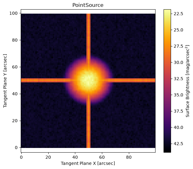
Point Source using PSFImage

M = ap.Model(
    model_type="point model",
    center=[50, 50],
    flux=10,
    psf=psf_target,
    target=basic_target,
)
M.initialize()
M.to()

fig, ax = plt.subplots(figsize=(7, 6))
ap.plots.model_image(fig, ax, M)
ax.set_title(M.name)
plt.show()

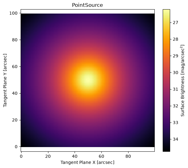
Point Source using PSF model

psf = ap.Model(model_type="moffat psf model", n=2.0, Rd=10.0, target=psf_target)
psf.initialize()

M = ap.Model(
    model_type="point model",
    center=[50, 50],
    flux=1,
    psf=psf,
    target=basic_target,
)
M.initialize()
print(M)
fig, ax = plt.subplots(figsize=(7, 6))
ap.plots.model_image(fig, ax, M)
ax.set_title(M.name)
plt.show()

PointSource|PointSource
    TargetImage|TargetImage
        crtan|static: [0, 0]
        crval|static: [0, 0]
        CD|static: [[1, 0], [0, 1]]
    center|dynamic: [50, 50]
    flux|dynamic: 1
    MoffatPSF|MoffatPSF
        center|static: [0, 0]
        n|dynamic: 2
        Rd|dynamic: 10
        I0|static: 1

Primary Galaxy Models

These models are represented mostly by their radial profile and are numerically straightforward to work with. All of these models also have perturbative extensions described below in the SuperEllipse, Fourier, Warp, Ray, and Wedge sections.

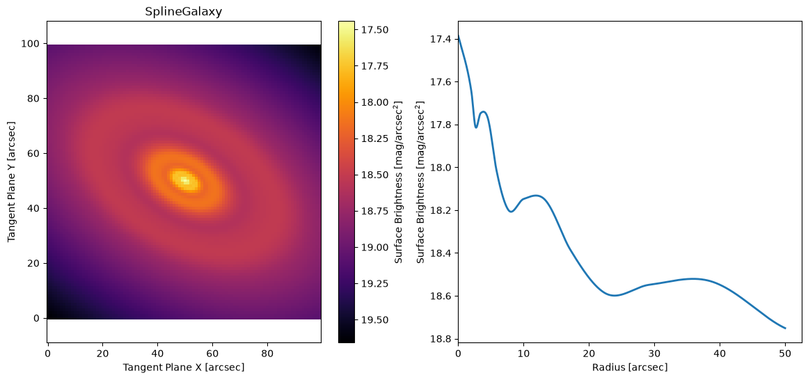
Spline Galaxy Model

This model has a radial surface brightness profile which can take on any function (that can be represented as a spline). This is somewhat like elliptical isophote fitting, though it is more precise in its definition of the SB model.

# Here we make an arbitrary spline profile out of a sine wave and a line
x = np.linspace(0, 10, 14)
spline_profile = np.array(list((np.sin(x * 2 + 2) / 20 + 1 - x / 20)) + [-4])
# Here we write down some corresponding radii for the points in the non-parametric profile. AstroPhot will make
# radii to match an input profile, but it is generally better to manually provide values so you have some control
# over their placement. Just note that it is assumed the first point will be at R = 0.
NP_prof = [0] + list(np.logspace(np.log10(2), np.log10(50), 13)) + [200]

M = ap.Model(
    model_type="spline galaxy model",
    center=[50, 50],
    q=0.6,
    PA=60 * np.pi / 180,
    I_R={"value": 10**spline_profile, "prof": NP_prof},
    target=basic_target,
)
M.initialize()

fig, ax = plt.subplots(1, 2, figsize=(14, 6))
ap.plots.model_image(fig, ax[0], M)
ap.plots.radial_light_profile(fig, ax[1], M)
ax[0].set_title(M.name)
plt.show()

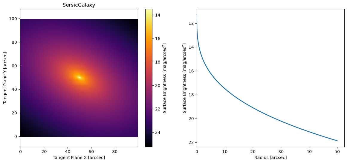
Sersic Galaxy Model

M = ap.Model(
    model_type="sersic galaxy model",
    center=[50, 50],
    q=0.6,
    PA=60 * np.pi / 180,
    n=3,
    Re=10,
    Ie=10,
    target=basic_target,
)
M.initialize()

fig, ax = plt.subplots(1, 2, figsize=(14, 6))
ap.plots.model_image(fig, ax[0], M)
ap.plots.radial_light_profile(fig, ax[1], M)
ax[0].set_title(M.name)
plt.show()

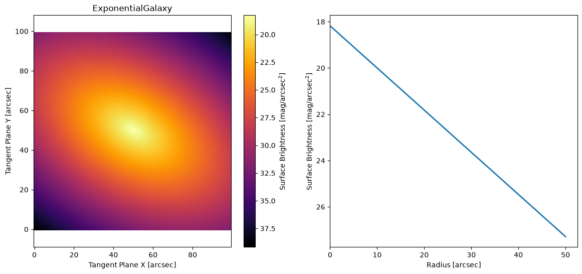
Exponential Galaxy Model

M = ap.Model(
    model_type="exponential galaxy model",
    center=[50, 50],
    q=0.6,
    PA=60 * np.pi / 180,
    Re=10,
    Ie=1,
    target=basic_target,
)
M.initialize()

fig, ax = plt.subplots(1, 2, figsize=(14, 6))
ap.plots.model_image(fig, ax[0], M)
ap.plots.radial_light_profile(fig, ax[1], M)
ax[0].set_title(M.name)
plt.show()

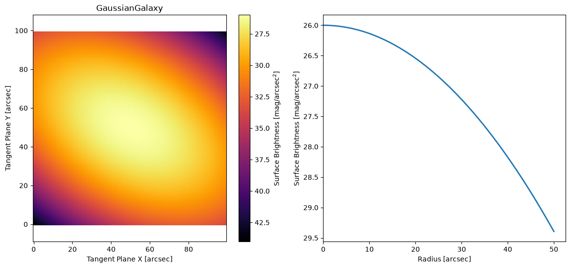
Gaussian Galaxy Model

M = ap.Model(
    model_type="gaussian galaxy model",
    center=[50, 50],
    q=0.6,
    PA=60 * np.pi / 180,
    sigma=20,
    flux=10,
    target=basic_target,
)
M.initialize()

fig, ax = plt.subplots(1, 2, figsize=(14, 6))
ap.plots.model_image(fig, ax[0], M)
ap.plots.radial_light_profile(fig, ax[1], M)
ax[0].set_title(M.name)
plt.show()

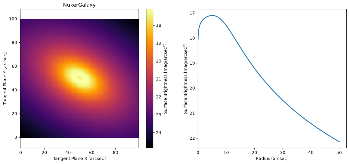
Nuker Galaxy Model

M = ap.Model(
    model_type="nuker galaxy model",
    center=[50, 50],
    q=0.6,
    PA=60 * np.pi / 180,
    Rb=10.0,
    Ib=10.0,
    alpha=4.0,
    beta=3.0,
    gamma=-0.2,
    target=basic_target,
)
M.initialize()

fig, ax = plt.subplots(1, 2, figsize=(14, 6))
ap.plots.model_image(fig, ax[0], M)
ap.plots.radial_light_profile(fig, ax[1], M)
ax[0].set_title(M.name)
plt.show()

/home/docs/checkouts/readthedocs.org/user_builds/astrophot/envs/stable/lib/python3.12/site-packages/astrophot/utils/conversions/units.py:29: RuntimeWarning: divide by zero encountered in log10
  return -2.5 * np.log10(flux) + zeropoint + 2.5 * np.log10(pixel_area)

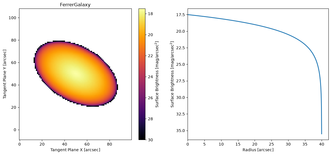
Ferrer Model

M = ap.Model(
    model_type="ferrer galaxy model",
    center=[50, 50],
    q=0.6,
    PA=60 * np.pi / 180,
    rout=40.0,
    alpha=2.0,
    beta=1.0,
    I0=10.0,
    target=basic_target,
)
M.initialize()

fig, ax = plt.subplots(1, 2, figsize=(14, 6))
ap.plots.model_image(fig, ax[0], M, vmax=30)
ap.plots.radial_light_profile(fig, ax[1], M)
ax[0].set_title(M.name)
plt.show()

/home/docs/checkouts/readthedocs.org/user_builds/astrophot/envs/stable/lib/python3.12/site-packages/astrophot/utils/conversions/units.py:29: RuntimeWarning: divide by zero encountered in log10
  return -2.5 * np.log10(flux) + zeropoint + 2.5 * np.log10(pixel_area)

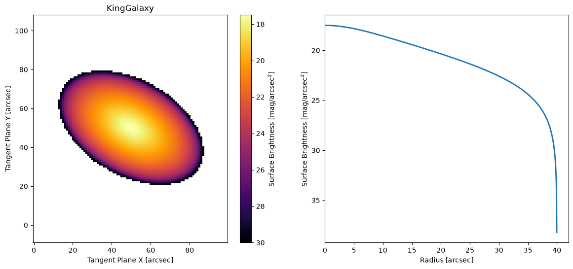
King Model

This is the Empirical King model with the extra free parameter \(\alpha\)

M = ap.Model(
    model_type="king galaxy model",
    center=[50, 50],
    q=0.6,
    PA=60 * np.pi / 180,
    Rc=10.0,
    Rt=40.0,
    alpha=2.01,
    I0=10.0,
    target=basic_target,
)
M.initialize()

fig, ax = plt.subplots(1, 2, figsize=(14, 6))
ap.plots.model_image(fig, ax[0], M, vmax=30)
ap.plots.radial_light_profile(fig, ax[1], M)
ax[0].set_title(M.name)
plt.show()

/home/docs/checkouts/readthedocs.org/user_builds/astrophot/envs/stable/lib/python3.12/site-packages/astrophot/utils/conversions/units.py:29: RuntimeWarning: divide by zero encountered in log10
  return -2.5 * np.log10(flux) + zeropoint + 2.5 * np.log10(pixel_area)

Special Galaxy Models

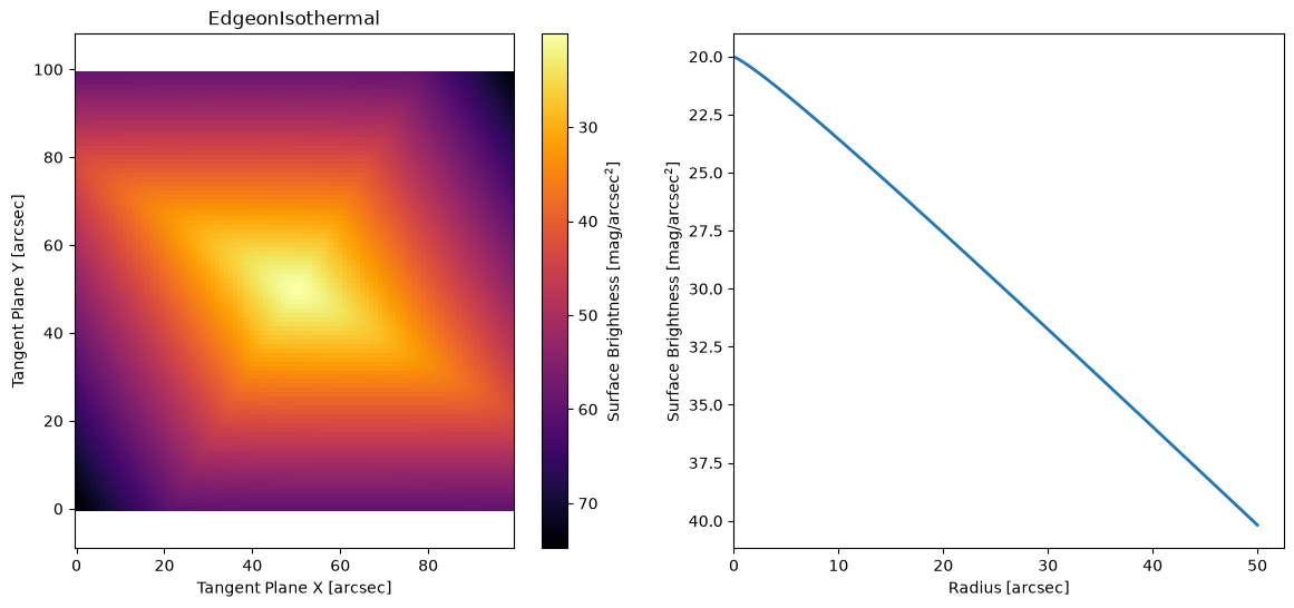
Edge on model

Currently there is only one dedicared edge on model, the self gravitating isothermal disk from van der Kruit & Searle 1981. If you know of another common edge on model, feel free to let us know and we can add it in!

M = ap.Model(
    model_type="isothermal sech2 edgeon model",
    center=[50, 50],
    PA=60 * np.pi / 180,
    I0=1.0,
    hs=3.0,
    rs=5.0,
    target=basic_target,
)
M.initialize()

fig, ax = plt.subplots(1, 2, figsize=(14, 6))
ap.plots.model_image(fig, ax[0], M)
ap.plots.radial_light_profile(fig, ax[1], M)
ax[0].set_title(M.name)
plt.show()

/home/docs/checkouts/readthedocs.org/user_builds/astrophot/envs/stable/lib/python3.12/site-packages/astrophot/utils/conversions/units.py:29: RuntimeWarning: divide by zero encountered in log10
  return -2.5 * np.log10(flux) + zeropoint + 2.5 * np.log10(pixel_area)

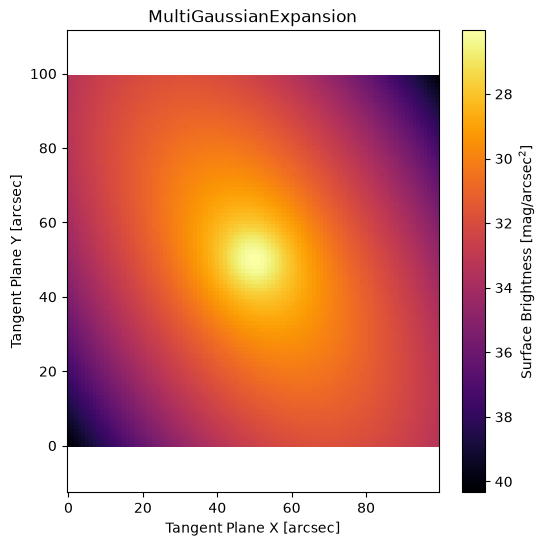
Multi Gaussian Expansion

A multi gaussian expansion is essentially a model made of overlapping gaussian models that share the same center. However, they are combined into a single model for computational efficiency. Another advantage of the MGE is that it is possible to determine a deprojection of the model from 2D into a 3D shape since the projection of a 3D gaussian is a 2D gaussian. Note however, that in some configurations this deprojection is not unique. See Cappellari 2002 for more details.

Note: The PA can be either a single value (same for all components) or an array with values for each component.

M = ap.Model(
    model_type="mge model",
    center=[50, 50],
    q=[0.9, 0.8, 0.6, 0.5],
    PA=30 * np.pi / 180,
    sigma=[4.0, 8.0, 16.0, 32.0],
    flux=np.ones(4) / 4,
    target=basic_target,
)
M.initialize()

fig, ax = plt.subplots(1, 1, figsize=(6, 6))
ap.plots.model_image(fig, ax, M)
ax.set_title(M.name)
plt.show()

Gaussian Ellipsoid

This model is an intrinsically 3D gaussian ellipsoid shape, which is projected to 2D for imaging.

M = ap.Model(
    model_type="gaussianellipsoid model",
    center=[50, 50],
    sigma_a=20.0,  # disk radius
    sigma_b=20.0,  # also disk radius
    sigma_c=2.0,  # disk thickness
    alpha=0.0,  # disk spin
    beta=np.arccos(0.6),  # disk inclination
    gamma=30 * np.pi / 180,  # disk position angle
    flux=10.0,
    target=basic_target,
)
M.initialize()

Show code cell source

Hide code cell source

beta = np.linspace(0, np.pi, 50)
M.beta = beta[0]
fig, ax = plt.subplots(1, 1, figsize=(6, 6))
ap.plots.model_image(fig, ax, M, showcbar=False)


def update(frame):
    M.beta = beta[frame]
    ax.clear()
    ap.plots.model_image(fig, ax, M, showcbar=False, vmin=24, vmax=30)
    ax.set_title(f"{M.name} beta = {beta[frame]:.2f} rad")
    return ax


ani = animation.FuncAnimation(fig, update, frames=50, interval=60)
plt.close()
# Save animation as gif
# ani.save("microlensing_animation.gif", writer='pillow', fps=16)  # Adjust 'fps' for the speed
# Or display the animation inline
HTML(ani.to_jshtml())

Animation.save using <class 'matplotlib.animation.HTMLWriter'>

Once Loop Reflect

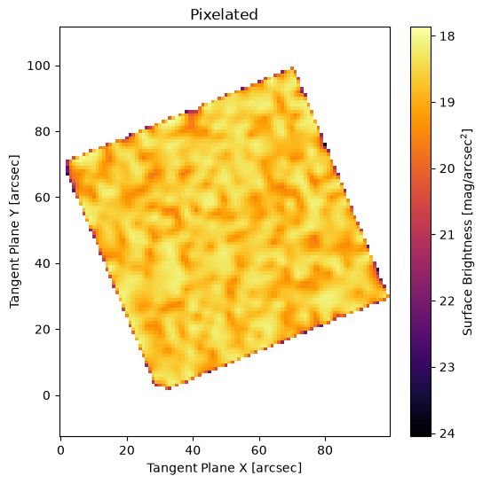
Pixelated Model

This model is simply a 2D grid of pixels which will be bilinearly interpolated to create the model on the sky. This can get out of hand quickly in terms of the number of parameters, so be careful!

M = ap.Model(
    model_type="pixelated model",
    center=[50, 50],
    I=np.random.uniform(0, 5, (25, 25)) + 1,
    PA=np.pi / 8,
    scale=3,
    target=basic_target,
)
M.initialize()

fig, ax = plt.subplots(1, 1, figsize=(6, 6))
ap.plots.model_image(fig, ax, M)
ax.set_title(M.name)
plt.show()

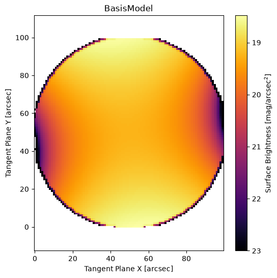
Basis Model

This model is similar to the pixelated model, except instead of having the pixels as part of the model, you provide a series of pixelated images as a basis and the model parameters are scalar weights multiplied by the basis. Think eigen decomposition, or zernike polynomials, or wavelets/shapelets. This is just like the BasisPSF model except intended for extended sources.

Currently just zernike:n is available as an option for automatic basis construction, but you can provide any set of images and use those instead!

weights = [2, 0.0, 0.0, -0.5, 0.0, 2.0]
M = ap.Model(
    model_type="basis model",
    basis="zernike:2",
    center=[50, 50],
    weights=weights,
    target=basic_target,
)

M.initialize()

fig, ax = plt.subplots(1, 1, figsize=(6, 6))
ap.plots.model_image(fig, ax, M, vmax=23)
ax.set_title(M.name)
plt.show()

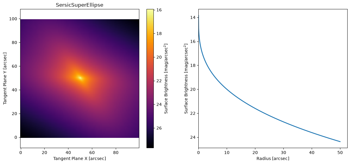
Super Ellipse Models

A super ellipse is a regular ellipse, except the radius metric changes from \(R = \sqrt{x^2 + y^2}\) to the more general: \(R = |x^C + y^C|^{1/C}\). The parameter \(C = 2\) for a regular ellipse, for \(0<C<2\) the shape becomes more “disky” and for \(C > 2\) the shape becomes more “boxy.”

There are superellipse versions of all the primary galaxy models: sersic, exponential, gaussian, moffat, spline, ferrer, king, and nuker

Sersic SuperEllipse

M = ap.Model(
    model_type="sersic superellipse galaxy model",
    center=[50, 50],
    q=0.6,
    PA=60 * np.pi / 180,
    C=4,
    n=3,
    Re=10,
    Ie=1,
    target=basic_target,
)
M.initialize()

fig, ax = plt.subplots(1, 2, figsize=(14, 6))
ap.plots.model_image(fig, ax[0], M)
ap.plots.radial_light_profile(fig, ax[1], M)
ax[0].set_title(M.name)
plt.show()

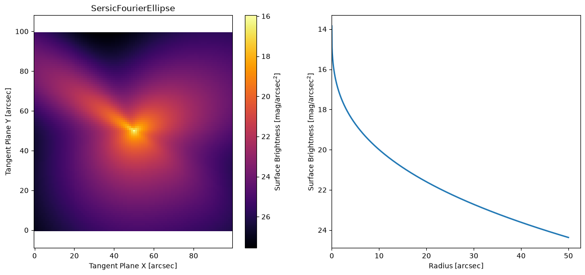
Fourier Ellipse Models

A Fourier ellipse is a scaling on the radius values as a function of theta. It takes the form: \(R' = R * \exp(\sum_m a_m*\cos(m*\theta + \phi_m))\), where am and phim are the parameters which describe the Fourier perturbations. Using the “modes” argument as a tuple, users can select which Fourier modes are used. As a rough intuition: mode 1 acts like a shift of the model; mode 2 acts like ellipticity; mode 3 makes a lopsided model (triangular in the extreme); and mode 4 makes peanut/diamond perturbations.

There are Fourier Ellipse versions of all the primary galaxy models: sersic, exponential, gaussian, moffat, spline, ferrer, king, and nuker

Sersic Fourier

fourier_am = np.array([0.1, 0.3, -0.2])
fourier_phim = np.array([10 * np.pi / 180, 0, 40 * np.pi / 180])

M = ap.Model(
    model_type="sersic fourier galaxy model",
    center=[50, 50],
    q=0.6,
    PA=60 * np.pi / 180,
    am=fourier_am,
    phim=fourier_phim,
    modes=(2, 3, 4),
    n=3,
    Re=10,
    Ie=1,
    target=basic_target,
)
M.initialize()

fig, ax = plt.subplots(1, 2, figsize=(14, 6))
ap.plots.model_image(fig, ax[0], M)
ap.plots.radial_light_profile(fig, ax[1], M)
ax[0].set_title(M.name)
plt.show()

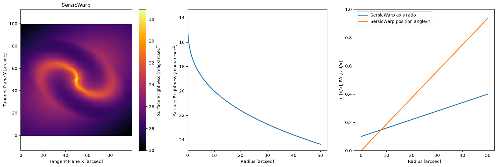
Warp Model

A warp model performs a radially varying coordinate transform. Essentially instead of applying a rotation matrix Rot on all coordinates X,Y we instead construct a unique rotation matrix for each coordinate pair Rot(R) where \(R = \sqrt{X^2 + Y^2}\). We also apply a radially dependent axis ratio q(R) to all the coordinates:

\(R = \sqrt{X^2 + Y^2}\)

\(X, Y = Rotate(X, Y, PA(R))\)

\(Y = \frac{Y}{q(R)}\)

The net effect is a radially varying PA and axis ratio which allows the model to represent spiral arms, bulges, or other features that change the apparent shape of a galaxy in a radially varying way.

There are warp versions of all the primary galaxy models: sersic, exponential, gaussian, moffat, spline, ferrer, king, and nuker

Sersic Warp

warp_q = np.linspace(0.1, 0.4, 14)
warp_pa = np.linspace(0, np.pi - 0.2, 14)
prof = np.linspace(0.0, 50, 14)
M = ap.Model(
    model_type="sersic warp galaxy model",
    center=[50, 50],
    q=0.6,
    PA=60 * np.pi / 180,
    q_R={"value": warp_q, "dynamic": True, "prof": prof},
    PA_R={"value": warp_pa, "dynamic": True, "prof": prof},
    n=3,
    Re=10,
    Ie=1,
    target=basic_target,
)
M.initialize()

fig, ax = plt.subplots(1, 3, figsize=(20, 6))
ap.plots.model_image(fig, ax[0], M)
ap.plots.radial_light_profile(fig, ax[1], M)
ap.plots.warp_phase_profile(fig, ax[2], M)
ax[2].legend()
ax[0].set_title(M.name)
plt.show()

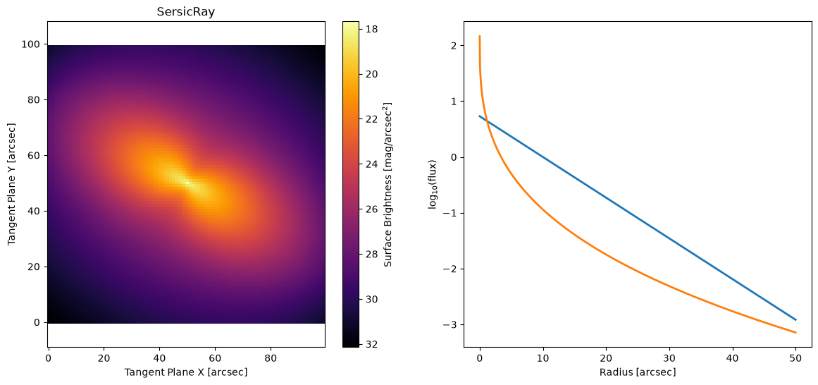
Ray Model

A ray model allows the user to break the galaxy up into regions that can be fit separately. There are two basic kinds of ray model: symmetric and asymmetric. A symmetric ray model (symmetric_rays = True) assumes 180 degree symmetry of the galaxy and so each ray is reflected through the center. This means that essentially the major axes and the minor axes are being fit separately. For an asymmetric ray model (symmetric_rays = False) each ray is it’s own profile to be fit separately.

In a ray model there is a smooth boundary between the rays. This smoothness is accomplished by applying a \((\cos(r*theta)+1)/2\) weight to each profile, where r is dependent on the number of rays and theta is shifted to center on each ray in turn. The exact cosine weighting is dependent on if the rays are symmetric and if there is an even or odd number of rays.

There are ray versions of all the primary galaxy models: sersic, exponential, gaussian, moffat, spline, ferrer, king, and nuker

Sersic Ray

M = ap.Model(
    model_type="sersic ray galaxy model",
    symmetric=True,
    segments=2,
    center=[50, 50],
    q=0.6,
    PA=60 * np.pi / 180,
    n=[1, 3],
    Re=[10, 5],
    Ie=[1, 0.5],
    target=basic_target,
)
M.initialize()

fig, ax = plt.subplots(1, 2, figsize=(14, 6))
ap.plots.model_image(fig, ax[0], M)
ap.plots.ray_light_profile(fig, ax[1], M)
ax[0].set_title(M.name)
plt.show()

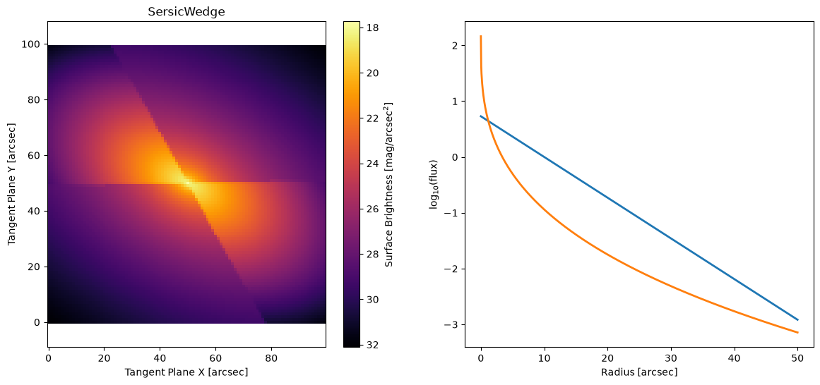
Wedge Model

A wedge model behaves just like a ray model, except the boundaries are sharp. This has the advantage that the wedges can be very different in brightness without the “smoothing” from the ray model washing out the dimmer one. It also has the advantage of less “mixing” of information between the rays, each one can be counted on to have fit only the pixels in it’s wedge without any influence from a neighbor. However, it has the disadvantage that the discontinuity at the boundary makes fitting behave strangely when a bright spot lays near the boundary.

There are wedge versions of all the primary galaxy models: sersic, exponential, gaussian, moffat, spline, ferrer, king, and nuker

Sersic Wedge

M = ap.Model(
    model_type="sersic wedge galaxy model",
    symmetric=True,
    segments=2,
    center=[50, 50],
    q=0.6,
    PA=60 * np.pi / 180,
    n=[1, 3],
    Re=[10, 5],
    Ie=[1, 0.5],
    target=basic_target,
)
M.initialize()

fig, ax = plt.subplots(1, 2, figsize=(14, 6))
ap.plots.model_image(fig, ax[0], M)
ap.plots.ray_light_profile(fig, ax[1], M)
ax[0].set_title(M.name)
plt.show()

Batched Models

Batching a model means turning the evaluation of the model itself into a vectorized operation. All AstroPhot models can be batched over their parameters to produce variations on the same model. This is done roughly like this:

x0 = model.get_values()
x0_batched = torch.stack([x0, x0*1.1, x0*0.9]) # basically turn into vector of param vectors
results = torch.vmap(lambda x: model(x).data)(x0_batched)

and now results will be output images from the model, except with an extra dimension for all the parameter variations you tried.

This is super useful for things like running multiple chains in an MCMC, but sometimes we want other variations to allow for vectorization in sampling the model itself. This is where you use batch models.

Note: Once you put a model into a batched model, it generally becomes unusable. You should consider it as part of the configuration of the batch model, and now that is all you work with.

WARNING: Any model parameter you wish to batch over must be set to dynamic=True (by default most already are), see caskade hierarchical models for more details.

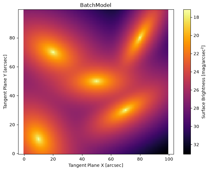
BatchModel

Any individual component model can be turned into a batch of models by wrapping it in the BatchModel class. This lets you represent a collection of similar objects/components in the same window.

This is computationally faster than creating a separate model for each object. Because of the constraints of the BatchModel it is able to do PSF convolution just once, on the summed image and so can get considerable performance enhancement.

M0 = ap.Model(
    model_type="sersic galaxy model",
    center=[50, 50],
    q=0.6,
    PA=60 * np.pi / 180,
    n=2,
    Re=5,
    Ie=1,
    target=basic_target,
)
M0.initialize()

M = ap.Model(model_type="batch model", model=M0)
# Now any parameters may be given an extra dimension for the batch
M0.center = [[10, 10], [20, 70], [50, 50], [70, 30], [80, 80]]
M0.q = [0.7, 0.6, 0.5, 0.4, 0.3]
M0.PA = np.array([30, 60, 90, 120, 150]) * np.pi / 180
# Parameters with single values will have the same value for all models

fig, ax = plt.subplots(figsize=(8, 6))
ap.plots.model_image(fig, ax, M)
ax.set_title(M.name)
plt.show()

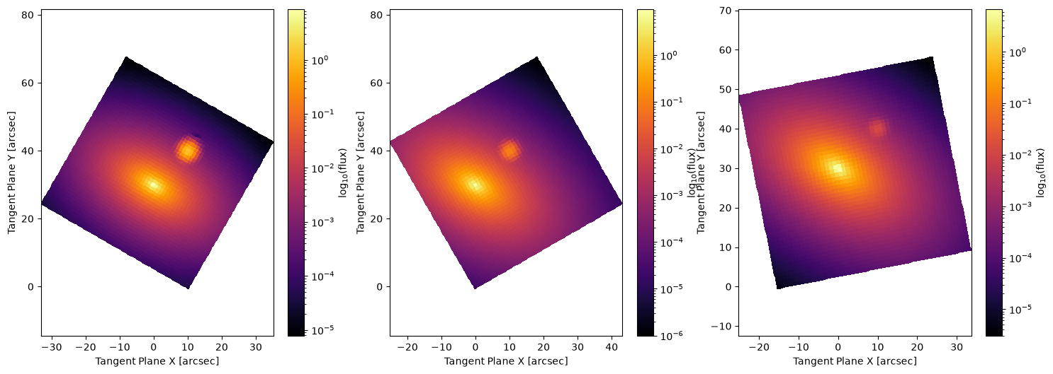
BatchSceneModel

Any AstroPhot component model or group model (but not a batched model) can be turned into a BatchSceneModel, which broadly lets you fit a single model over many images. This can be useful for fitting dithered images since it is the same scene being fit to a few slightly shifted images. This can also be useful for fitting transients embedded in a static host. It is possible to select which parameters will vary across all images and which will be fixed for all images.

target_batch = ap.TargetImageBatch(
    images=[
        ap.TargetImage(
            data=np.zeros((50, 50)),
            CD=ap.utils.initialize.R(np.pi / 3),
            crtan=(10, 0),
            name="image1",
        ),
        ap.TargetImage(data=np.zeros((50, 50)), CD=ap.utils.initialize.R(np.pi / 6), name="image2"),
        ap.TargetImage(
            data=np.zeros((50, 50)),
            CD=ap.utils.initialize.R(np.pi / 16),
            crtan=(-15, 0),
            name="image3",
        ),
    ]
)

M0_host = ap.Model(
    model_type="sersic galaxy model",
    center=[0, 30],
    q=0.6,
    PA=60 * np.pi / 180,
    n=2,
    Re=3,
    Ie=1,
    target=target_batch.images[0],  # can be any of them
)
M0_sn = ap.Model(
    model_type="point model",
    center=[10, 40],
    flux=1,
    psf=ap.utils.initialize.gaussian_psf(1.0, 11, 1.0),
    target=target_batch.images[0],
)
M0 = ap.Model(model_type="group model", models=[M0_host, M0_sn], target=target_batch.images[0])
M0.initialize()
M0_sn.flux = [10, 1, 0.1]  # we can give the SN different fluxes in each image

M = ap.Model(model_type="batch scene model", model=M0, target=target_batch)

fig, axarr = plt.subplots(1, 3, figsize=(18, 6))
ap.plots.model_image(fig, axarr, M)
plt.show()

PSF provided to PointSource was not a PSFImage or Model instance, so it was converted to a PSFImage assuming no upsampling.

Initializing model SersicGalaxy

Initializing model PointSource