Advanced PSF modeling

Ideally we always have plenty of well separated bright, but not oversaturated, stars to use to construct a PSF model. These models are incredibly important for certain science objectives that rely on precise shape measurements or even just total light measures. Here we demonstrate some of the special capabilities AstroPhot has to handle challenging scenarios where a good PSF model is needed but there are only very faint stars, poorly placed stars, or even no stars to work with!

Something to keep in mind, AstroPhot PSF models operate in pixel space. The PSFImage has no way to transform coordinates between the world, tangent plane, and pixel space, it only understands pixels. For this reason, if you check the units on any PSFModel parameters, they will be in pix units which are pixels in the target image. If the PSFModel is in an upsampled space, the units are still pixels in the target image (though everything will be sampled more finely).

%matplotlib inline
import astrophot as ap
import numpy as np
import torch
import matplotlib.pyplot as plt

Making a PSF model

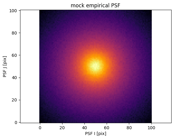
Before we can optimize a PSF model, we need to make the model and get some starting parameters. If you already have a good guess at some starting parameters then you can just enter them yourself, however if you don’t then AstroPhot provides another option; if you have an empirical PSF estimate (a stack of a few stars from the field), then you can have a PSF model initialize itself on the empirical PSF just like how other AstroPhot models can initialize themselves on target images. Let’s see how that works!

# First make a mock empirical PSF image
np.random.seed(124)
psf = ap.utils.initialize.moffat_psf(2.0, 3.0, 101, 0.5)
variance = psf**2 / 100
psf += np.random.normal(scale=np.sqrt(variance))

psf_target = ap.PSFImage(
    data=psf,
    upsample=1,
    variance=variance,
)

# To ensure the PSF has a normalized flux of 1, we call
psf_target.normalize()

fig, ax = plt.subplots()
ap.plots.psf_image(fig, ax, psf_target)
ax.set_title("mock empirical PSF")
plt.show()

# Now we initialize on the image
psf_model = ap.Model(
    name="init_psf",
    model_type="moffat psf model",
    target=psf_target,
)
psf_model.initialize()

# PSF model can be fit to it's own target for good initial values
ap.fit.LM(psf_model, verbose=1).fit()

fig, ax = plt.subplots(1, 2, figsize=(13, 5))
ap.plots.psf_image(fig, ax[0], psf_model)
ax[0].set_title("PSF model fit to mock empirical PSF")
ap.plots.residual_image(fig, ax[1], psf_model, normalize_residuals=True)
ax[1].set_title("residuals")
plt.show()

==Starting LM fit for 'init_psf' with 2 dynamic parameters and 10201 pixels==

Chi^2/DoF: 9.70669, L: 1

/home/docs/checkouts/readthedocs.org/user_builds/astrophot/envs/v0.17.3/lib/python3.12/site-packages/torch/jit/_script.py:1488: DeprecationWarning: `torch.jit.script` is deprecated. Please switch to `torch.compile` or `torch.export`.
  warnings.warn(

Chi^2/DoF: 1.15654, L: 1

Chi^2/DoF: 1.00834, L: 0.0123

Chi^2/DoF: 0.974047, L: 0.000152

Chi^2/DoF: 0.973718, L: 2.32e-08

Final Chi^2/DoF: 0.973718, L: 2.32e-08. Converged: success

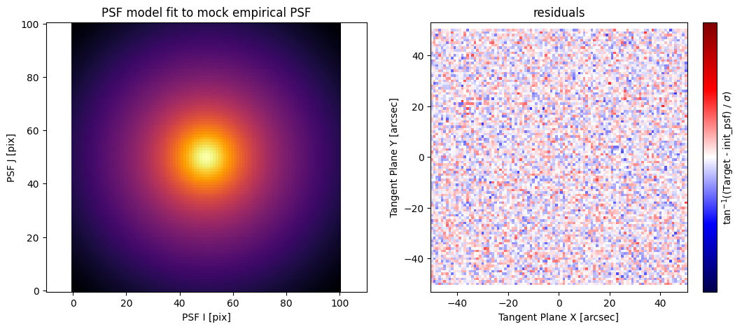
That’s pretty good! it doesn’t need to be perfect, so this is already in the right ballpark, just based on the size of the main light concentration. For the examples below, we will just start with some simple given initial parameters, but for real analysis this is quite handy.

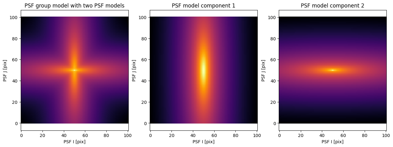
Group PSF Model

Just like group models for regular models, it is possible to make a psf group model to combine multiple psf models.

psf_model1 = ap.Model(
    name="psf1",
    model_type="moffat ellipse psf model",
    n=2,
    Rd=10,
    I0=2,  # essentially controls relative flux of this component
    PA=0,
    q=0.2,
    target=psf_target,
)
psf_model2 = ap.Model(
    name="psf2",
    model_type="sersic ellipse psf model",
    n=4,
    Re=5,
    Ie=1,
    PA=np.pi / 2,
    q=0.2,
    target=psf_target,
)
psf_group_model = ap.Model(
    name="psf_group",
    model_type="psf group model",
    target=psf_target,
    models=[psf_model1, psf_model2],
)
psf_group_model.initialize()
fig, ax = plt.subplots(1, 3, figsize=(15, 5))
ap.plots.psf_image(fig, ax[0], psf_group_model)
ax[0].set_title("PSF group model with two PSF models")
ap.plots.psf_image(fig, ax[1], psf_group_model.models[0])
ax[1].set_title("PSF model component 1")
ap.plots.psf_image(fig, ax[2], psf_group_model.models[1])
ax[2].set_title("PSF model component 2")
plt.show()

Initializing model psf1

Initializing model psf2

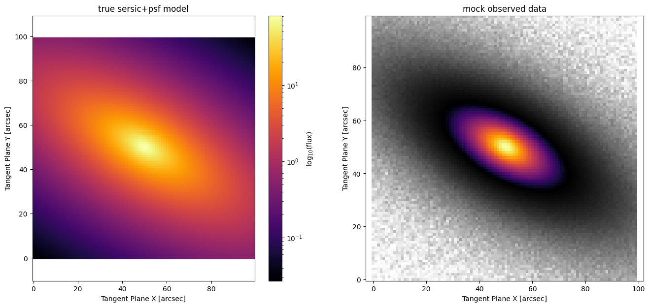
PSF modeling without stars

Can it be done? Let’s see!

# Lets make some data that we need to fit
psf_target = ap.PSFImage(data=np.zeros((51, 51)), upsample=1)

true_psf_model = ap.Model(
    name="true_psf",
    model_type="moffat psf model",
    target=psf_target,
    n=2,
    Rd=3,
    I0=1.0,
)
true_psf = true_psf_model().data

target = ap.TargetImage(data=torch.zeros(100, 100), psf=true_psf)

true_model = ap.Model(
    name="true_model",
    model_type="sersic galaxy model",
    target=target,
    center=[50.0, 50.0],
    q=0.4,
    PA=np.pi / 3,
    n=2,
    Re=25,
    Ie=10,
)

# use the true model to make some data
sample = true_model()._data
torch.manual_seed(61803398)
target._data = sample + torch.normal(torch.zeros_like(sample), 0.1)
target.variance = 0.01 * torch.ones_like(sample.T)

fig, ax = plt.subplots(1, 2, figsize=(16, 7))
ap.plots.model_image(fig, ax[0], true_model)
ap.plots.target_image(fig, ax[1], target)
ax[0].set_title("true sersic+psf model")
ax[1].set_title("mock observed data")
plt.show()

# Now we will try and fit the data using just a plain sersic

# Here we set up a sersic model for the galaxy
plain_galaxy_model = ap.Model(
    name="galaxy_model",
    model_type="sersic galaxy model",
    target=target,
    psf_convolve=False,
)

# Let AstroPhot determine its own initial parameters, so it has to start with whatever it decides automatically,
# just like a real fit.
plain_galaxy_model.initialize()

result = ap.fit.LM(plain_galaxy_model, verbose=1).fit()
print(result.message)

==Starting LM fit for 'galaxy_model' with 7 dynamic parameters and 10000 pixels==

Chi^2/DoF: 145.259, L: 1

Chi^2/DoF: 42.2055, L: 1

Chi^2/DoF: 28.7034, L: 1

Chi^2/DoF: 25.3748, L: 1

Chi^2/DoF: 22.8064, L: 0.00137

Chi^2/DoF: 22.7894, L: 2.32e-08

Final Chi^2/DoF: 22.7894, L: 2.32e-08. Converged: success

success

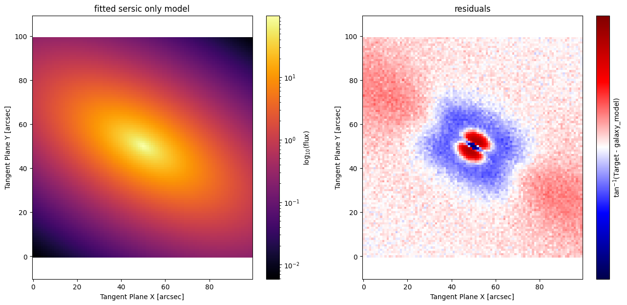
# The shape of the residuals here shows that there is still missing information; this is of course
# from the missing PSF convolution to blur the model. In fact, the shape of those residuals is very
# commonly seen in real observed data (ground based) when it is fit without accounting for PSF blurring.
fig, ax = plt.subplots(1, 2, figsize=(16, 7))
ap.plots.model_image(fig, ax[0], plain_galaxy_model)
ap.plots.residual_image(fig, ax[1], plain_galaxy_model)
ax[0].set_title("fitted sersic only model")
ax[1].set_title("residuals")
plt.show()

# Now we will try and fit the data with a sersic model and a "live" psf

# Here we create a target psf model which will determine the specs of our live psf model
psf_target = ap.PSFImage(data=np.zeros((51, 51)))

live_psf_model = ap.Model(
    name="psf",
    model_type="moffat psf model",
    target=psf_target,
    n=1.0,  # True value is 2.
    Rd=2.0,  # True value is 3.
)

# Here we set up a sersic model for the galaxy
live_galaxy_model = ap.Model(
    name="galaxy_model",
    model_type="sersic galaxy model",
    target=target,
    psf=live_psf_model,  # Here we bind the PSF model to the galaxy model
)
live_galaxy_model.initialize()
print(live_galaxy_model)
print(live_galaxy_model.jacobian())
result = ap.fit.LM(live_galaxy_model, verbose=3).fit()

galaxy_model|SersicGalaxy
    TargetImage|TargetImage
        crtan|static: [0, 0]
        crval|static: [0, 0]
        CD|static: [[1, 0], [0, 1]]
    center|dynamic: [49.3, 49.9]
    q|dynamic: 0.488
    PA|dynamic: 0.919
    n|dynamic: 1.19
    Re|dynamic: 20.5
    Ie|dynamic: 12.4
    psf|MoffatPSF
        center|static: [0, 0]
        n|dynamic: 1
        Rd|dynamic: 2
        I0|static: 1
TargetImage_jacobian|JacobianImage
    crtan|static: [0, 0]
    crval|static: [0, 0]
    CD|static: [[1, 0], [0, 1]]
==Starting LM fit for 'galaxy_model' with 9 dynamic parameters and 10000 pixels==

Chi^2/DoF: 1184.78, L: 1

Chi^2/DoF: 266.978, L: 1

Chi^2/DoF: 28.1537, L: 1

Chi^2/DoF: 19.8643, L: 1

Chi^2/DoF: 17.7909, L: 1

Chi^2/DoF: 12.7104, L: 0.111

Chi^2/DoF: 10.7596, L: 0.111

Chi^2/DoF: 7.83639, L: 0.0123

Chi^2/DoF: 4.51998, L: 0.0123

Chi^2/DoF: 3.3578, L: 0.0123

Chi^2/DoF: 2.67986, L: 0.0123

Chi^2/DoF: 2.25382, L: 0.0123

Chi^2/DoF: 1.96897, L: 0.0123

Chi^2/DoF: 1.76986, L: 0.0123

Chi^2/DoF: 1.26037, L: 0.00137

Chi^2/DoF: 1.1059, L: 0.00137

Chi^2/DoF: 1.04704, L: 0.00137

Chi^2/DoF: 1.01998, L: 0.00137

Chi^2/DoF: 1.00693, L: 0.00137

Chi^2/DoF: 1.00039, L: 0.00137

Chi^2/DoF: 0.99653, L: 0.000152

Chi^2/DoF: 0.993114, L: 0.000152

Chi^2/DoF: 0.993063, L: 1.69e-05

Final Chi^2/DoF: 0.993063, L: 1.88e-06. Converged: success

print(
    f"fitted n for moffat PSF: {live_psf_model.n.value.item():.6f} +- {live_psf_model.n.uncertainty.item():.6f} we were hoping to get 2!"
)
print(
    f"fitted Rd for moffat PSF: {live_psf_model.Rd.value.item():.6f} +- {live_psf_model.Rd.uncertainty.item():.6f} we were hoping to get 3!"
)
fig, ax = ap.plots.covariance_matrix(
    result.covariance_matrix.detach().cpu().numpy(),
    live_galaxy_model.get_values().detach().cpu().numpy(),
    live_galaxy_model.build_params_array_names(),
)
plt.show()

fitted n for moffat PSF: 2.006386 +- 0.012891 we were hoping to get 2!
fitted Rd for moffat PSF: 2.993695 +- 0.012316 we were hoping to get 3!

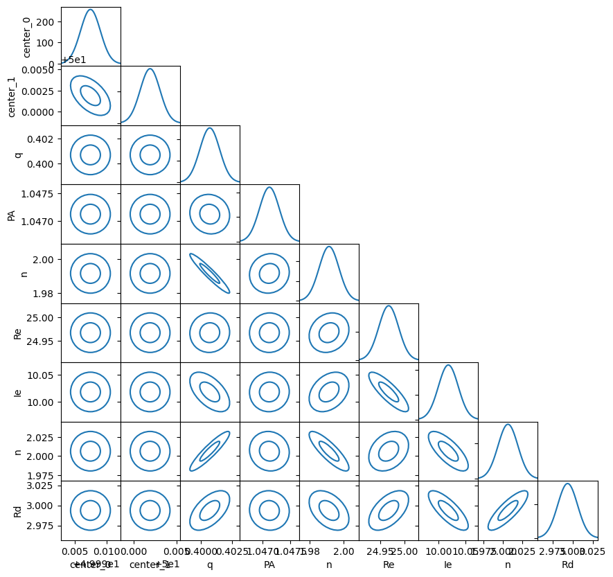
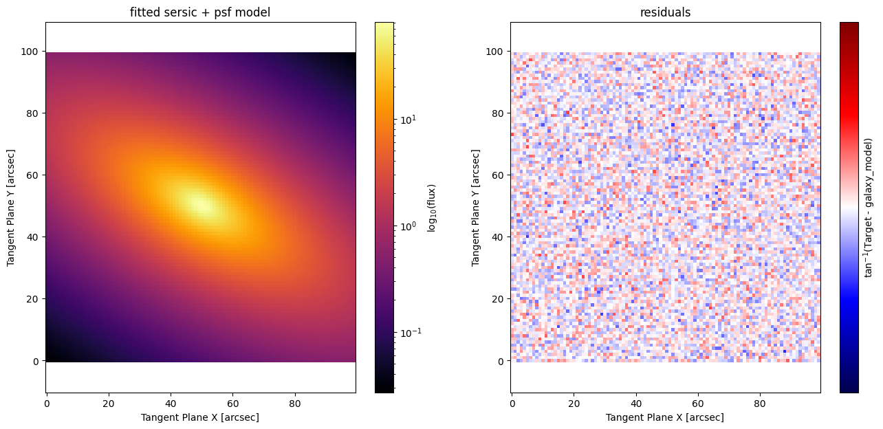
This is truly remarkable! With no stars available we were still able to extract an accurate PSF from the image! To be fair, this example is essentially perfect for this kind of fitting and we knew the true model types (sersic and moffat) from the start. Still, this is a powerful capability in certain scenarios. For many applications (e.g. weak lensing) it is essential to get the absolute best PSF model possible. Here we have shown that not only stars, but galaxies in the field can be useful tools for measuring the PSF!

fig, ax = plt.subplots(1, 2, figsize=(16, 7))
ap.plots.model_image(fig, ax[0], live_galaxy_model)
ap.plots.residual_image(fig, ax[1], live_galaxy_model)
ax[0].set_title("fitted sersic + psf model")
ax[1].set_title("residuals")
plt.show()

There are regions of parameter space that are degenerate and so even in this idealized scenario the PSF model can get stuck. If you rerun the notebook with different random number seeds for pytorch you may find some where the optimizer “fails by immobility” this is when it gets stuck in the parameter space and can’t find any way to improve the likelihood. In fact most of these “fail” fits do return really good values for the PSF model, so keep in mind that the “fail” flag only means the possibility of a truly failed fit. Unfortunately, detecting convergence is hard.

PSF fitting for faint stars

Sometimes there are stars available, but they are faint and it is hard to see how a reliable fit could be obtained. We have already seen how faint stars next to galaxies are still viable for PSF fitting. With AstroPhot joint modelling it is possible to share information between images, so a faint UV band can be informed by a well sampled r-band (for example). This will fix the positions of the stars very accurately. Then it is just a matter of combining enough stars to get enough signal for AstroPhot to run the fit, this takes fewer stars than you think because the centers are already essentially perfect.

PSF fitting for saturated stars

A saturated star is a bright star, and it’s just begging to be used for modelling a PSF. There’s just one catch, the highest signal to noise region is completely messed up and can’t be used! Traditionally these stars are either ignored, or a two stage fit is performed to get an “inner psf” and an “outer psf” which are then merged. Why not fit the inner and outer PSFs all at once! This can be done with AstroPhot using parameter constraints and masking. Simply mask the saturated data and fit a PSF model, AstroPhot will use the available information in the outskirts of the bright star. If you can add some faint stars to the fit then that will give AstroPhot a handle on the inner parts of the PSF. With everything fit jointly, the information is shared in one big likelihood calculation and it should converge to something very reasonable (though getting it set up may be finicky).

Keep in mind that it is common for the PSF to vary with brightness, so you may need to add a flux dependent component to the PSF model. This can be achieved using caskade parameter management. If you are having difficulties, just contact me and I’ll help you through it!