Getting Started with AstroPhot

In this notebook you will walk through the very basics of AstroPhot functionality. Here you will learn how to make models; how to set them up for fitting; and how to view the results. These core elements will come up every time you use AstroPhot, though in future notebooks you will learn how to take advantage of the advanced features in AstroPhot.

Note: AstroPhot is now a caskade ecosystem project, meaning its parameters have an incredible amount of flexibility. Check out the documentation for more details!

%matplotlib inline
%load_ext autoreload
%autoreload 2

import astrophot as ap
import numpy as np
import torch
from astropy.io import fits
from astropy.wcs import WCS
import matplotlib.pyplot as plt

Your first model

The basic format for making an AstroPhot model is given below. Once a model object is constructed, it can be manipulated and updated in various ways.

model1 = ap.Model(
    name="model1",
    model_type="sersic galaxy model",  # this specifies the kind of model
    # here we set initial values for each parameter
    center=[50, 50],
    q=0.6,
    PA=60 * np.pi / 180,
    n=2,
    Re=10,
    Ie=1,
    # every model needs a target, more on this later
    target=ap.TargetImage(data=np.zeros((100, 100)), zeropoint=22.5),
)

# models must/should be initialized before doing anything with them.
# This makes sure all the parameters and metadata are ready to go.
model1.initialize()

# We can print the model's current state
print(model1)

model1|SersicGalaxy
    TargetImage|TargetImage
        crtan|static: [0, 0]
        crval|static: [0, 0]
        CD|static: [[1, 0], [0, 1]]
    center|dynamic: [50, 50]
    q|dynamic: 0.6
    PA|dynamic: 1.05
    n|dynamic: 2
    Re|dynamic: 10
    Ie|dynamic: 1

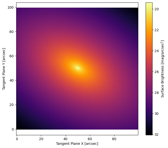
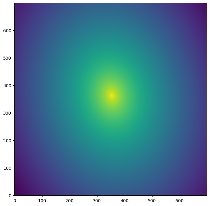
# AstroPhot has built in methods to plot relevant information. This plots the model
# as projected into the "target" image. Thus it has the same pixelscale, orientation
# and (optionally) PSF as the model's target.
fig, ax = plt.subplots(figsize=(8, 7))
ap.plots.model_image(fig, ax, model1)
plt.show()

Giving the model a Target

Typically, the main goal when constructing an AstroPhot model is to fit to an image. We need to give the model access to the image and some information about it to get started.

# first let's download an image to play with
############ UNCOMMENT IF RUNNING LOCALLY ############
# hdu = fits.open(
#     "https://www.legacysurvey.org/viewer/fits-cutout?ra=36.3684&dec=-25.6389&size=700&layer=ls-dr9&pixscale=0.262&bands=r"
# )
# hdu.writeto("target_image.fits", overwrite=True)
hdu = fits.open("target_image.fits")
target_data = np.array(hdu[0].data, dtype=np.float64)

target = ap.TargetImage(
    data=target_data,
    pixelscale=0.262,
    zeropoint=22.5,  # optionally, a zeropoint tells AstroPhot the pixel flux units
    variance="auto",  # Automatic variance estimate for testing and demo purposes only! In real analysis use weight maps, counts, gain, etc to compute variance!
)

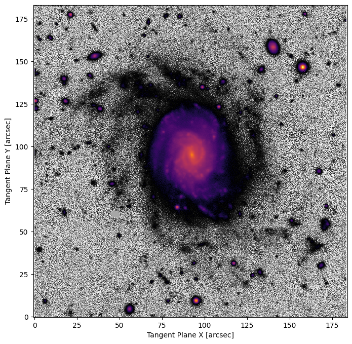
# The default AstroPhot target plotting method uses log scaling in bright areas and histogram scaling in faint areas
fig3, ax3 = plt.subplots(figsize=(8, 8))
ap.plots.target_image(fig3, ax3, target)
plt.show()

# This model now has a target that it will attempt to match
model2 = ap.Model(
    name="model_with_target",
    model_type="sersic galaxy model",
    target=target,
)

# Instead of giving initial values for all the parameters, it is possible to
# simply call "initialize" and AstroPhot will try to guess initial values for
# every parameter. It is also possible to set just a few parameters and let
# AstroPhot try to figure out the rest. For example you could give it an initial
# Guess for the center and it will work from there.
model2.initialize()

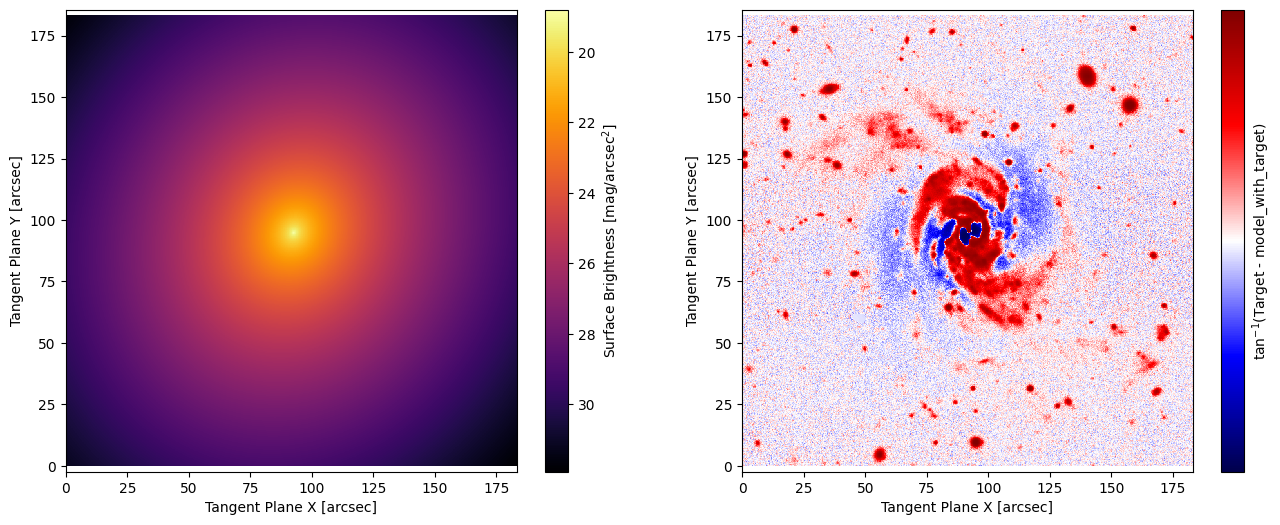
# Plotting the initial parameters and residuals, we see it gets the rough shape
# of the galaxy right, but still has some fitting to do
fig4, ax4 = plt.subplots(1, 2, figsize=(16, 6))
ap.plots.model_image(fig4, ax4[0], model2)
ap.plots.residual_image(fig4, ax4[1], model2)
plt.show()

# Now that the model has been set up with a target and initialized with parameter values, it is time to fit the image
result = ap.fit.LM(model2, verbose=1).fit()

# See that we use ap.fit.LM, this is the Levenberg-Marquardt Chi^2 minimization method, it is the recommended technique
# for most least-squares problems. See the Fitting Methods tutorial for more on fitters!
print("Fit message:", result.message)  # the fitter will store a message about its convergence

==Starting LM fit for 'model_with_target' with 7 dynamic parameters and 490000 pixels==

Chi^2/DoF: 7.46905, L: 1

/home/docs/checkouts/readthedocs.org/user_builds/astrophot/envs/v0.17.3/lib/python3.12/site-packages/torch/jit/_script.py:1488: DeprecationWarning: `torch.jit.script` is deprecated. Please switch to `torch.compile` or `torch.export`.
  warnings.warn(

Chi^2/DoF: 7.01169, L: 1

Chi^2/DoF: 6.84534, L: 0.111

Chi^2/DoF: 6.71701, L: 0.00137

Chi^2/DoF: 6.71123, L: 0.00137

Final Chi^2/DoF: 6.7112, L: 0.00137. Converged: success

Fit message: success

print(model2)
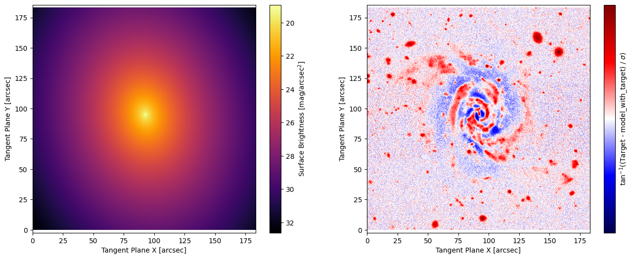
# we now plot the fitted model and the image residuals
fig5, ax5 = plt.subplots(1, 2, figsize=(16, 6))
ap.plots.model_image(fig5, ax5[0], model2)
ap.plots.residual_image(fig5, ax5[1], model2, normalize_residuals=True)
plt.show()

model_with_target|SersicGalaxy
    TargetImage|TargetImage
        crtan|static: [0, 0]
        crval|static: [0, 0]
        CD|static: [[0.262, 0], [0, 0.262]]
    center|dynamic: [92.7, 94.9]
    q|dynamic: 0.764
    PA|dynamic: 0.171
    n|dynamic: 1.64
    Re|dynamic: 14.6
    Ie|dynamic: 1.63

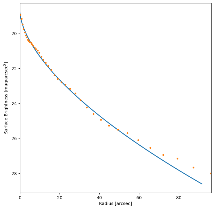
# Plot surface brightness profile

# we now plot the model profile and a data profile. The model profile is determined from the model parameters
# the data profile is determined by taking the median of pixel values at a given radius. Notice that the model
# profile is slightly higher than the data profile? This is because there are other objects in the image which
# are not being modelled, the data profile uses a median so they are ignored, but for the model we fit all pixels.
fig10, ax10 = plt.subplots(figsize=(8, 8))
ap.plots.radial_light_profile(fig10, ax10, model2)
ap.plots.radial_median_profile(fig10, ax10, model2)
plt.show()

Update uncertainty estimates

After running a fit, the ap.fit.LM optimizer can update the uncertainty for each parameter. In fact it can return the full covariance matrix if needed. For a demo of what can be done with the covariance matrix see the FittingMethods tutorial. One important note is that the variance image needs to be correct for the uncertainties to be meaningful!

result.update_uncertainty()
print(model2)

model_with_target|SersicGalaxy
    TargetImage|TargetImage
        crtan|static: [0, 0]
        crval|static: [0, 0]
        CD|static: [[0.262, 0], [0, 0.262]]
    center|dynamic: [92.7, 94.9]
    q|dynamic: 0.764
    PA|dynamic: 0.171
    n|dynamic: 1.64
    Re|dynamic: 14.6
    Ie|dynamic: 1.63

Note that these uncertainties are pure statistical uncertainties that come from evaluating the structure of the \(\chi^2\) minimum. Systematic uncertainties are not included and these often significantly outweigh the standard errors. As can be seen in the residual plot above, there is certainly plenty of unmodelled structure there. Use caution when interpreting the errors from these fits.

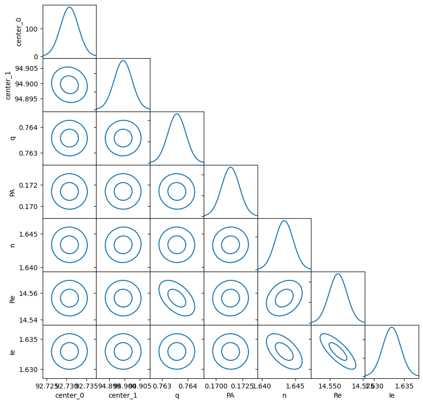
# Plot the uncertainty matrix

# While the scale of the uncertainty may not be meaningful if the image variance is not accurate, we
# can still see how the covariance of the parameters plays out in a given fit.
fig, ax = ap.plots.covariance_matrix(
    result.covariance_matrix.detach().cpu().numpy(),
    model2.get_values().detach().cpu().numpy(),
    model2.build_params_array_names(),
)
plt.show()

Record the total flux/magnitude

Often the parameter of interest is the total flux or magnitude, even if this isn’t one of the core parameters of the model, it can be computed. For Sersic and Moffat models with analytic total fluxes it will be integrated to infinity, for most other models it will simply be the total flux in the window.

print(
    f"Total Flux: {model2.total_flux().item():.1f} +- {model2.total_flux_uncertainty().item():.1f}"
)
print(
    f"Total Magnitude: {model2.total_magnitude().item():.4f} +- {model2.total_magnitude_uncertainty().item():.4f}"
)

Total Flux: 3921.7 +- 5.6

Total Magnitude: 13.5163 +- 0.0015

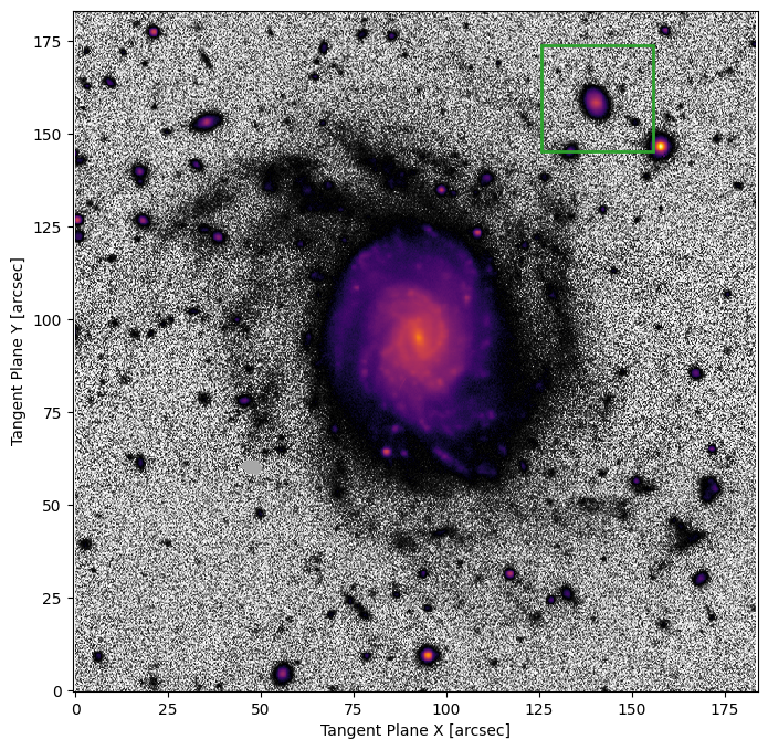
Giving the model a specific target window

Sometimes an object isn’t nicely centered in the image, and may not even be the dominant object in the image. It is therefore nice to be able to specify what part of the image we should analyze.

# note, we don't provide a name here. A unique name will automatically be generated using the model type
model3 = ap.Model(
    model_type="sersic galaxy model",
    target=target,
    window=[480, 595, 555, 665],  # this is a region in pixel coordinates (imin,imax,jmin,jmax)
)
print(f"automatically generated name: '{model3.name}'")

# We can plot the "model window" to show us what part of the image will be analyzed by that model
fig6, ax6 = plt.subplots(figsize=(8, 8))
ap.plots.target_image(fig6, ax6, model3.target)
ap.plots.model_window(fig6, ax6, model3)
plt.show()

automatically generated name: 'SersicGalaxy'

model3.initialize()
result = ap.fit.LM(model3, verbose=1).fit()

==Starting LM fit for 'SersicGalaxy' with 7 dynamic parameters and 12650 pixels==

Chi^2/DoF: 7.07561, L: 1

Chi^2/DoF: 4.67827, L: 1

Chi^2/DoF: 3.91608, L: 0.111

Chi^2/DoF: 3.44182, L: 0.111

Chi^2/DoF: 3.16322, L: 0.0123

Chi^2/DoF: 3.1581, L: 0.00137

Final Chi^2/DoF: 3.15809, L: 2.32e-08. Converged: success

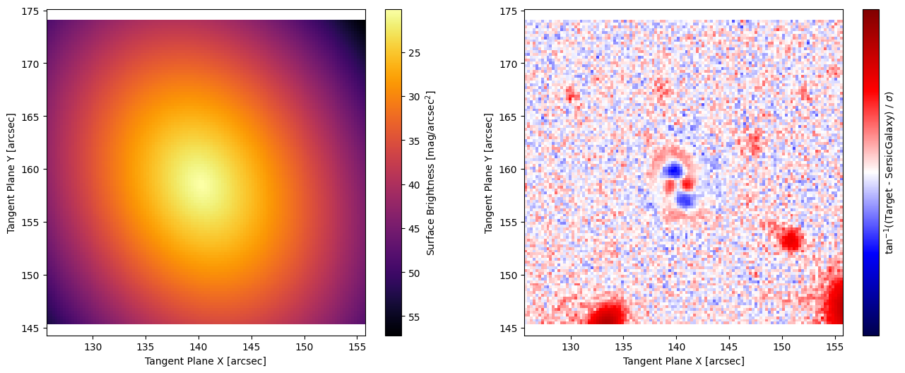
# Note that when only a window is fit, the default plotting methods will only show that window
print(model3)
fig7, ax7 = plt.subplots(1, 2, figsize=(16, 6))
ap.plots.model_image(fig7, ax7[0], model3)
ap.plots.residual_image(fig7, ax7[1], model3, normalize_residuals=True)
plt.show()

SersicGalaxy|SersicGalaxy
    TargetImage|TargetImage
        crtan|static: [0, 0]
        crval|static: [0, 0]
        CD|static: [[0.262, 0], [0, 0.262]]
    center|dynamic: [140, 159]
    q|dynamic: 0.771
    PA|dynamic: 0.398
    n|dynamic: 0.822
    Re|dynamic: 1.89
    Ie|dynamic: 2.55

Inspect parameters

AstroPhot is all about managing parameters, so there is lots of information that comes with them, lets see some of the meta-data you can access:

print("Parameter units, sersic Re:", model3.Re.units)
print("Expected parameter shape, Re:", model3.Re.shape)
print("and for center it is:", model3.center.shape)
print("Parameter dynamic state, Re:", model3.Re.dynamic, "so it will be optimized by a fitter")
print("Parameter description, Re:", model3.Re.description)

Parameter units, sersic Re: arcsec
Expected parameter shape, Re: ()
and for center it is: (2,)
Parameter dynamic state, Re: True so it will be optimized by a fitter
Parameter description, Re: half light radius, also called effective radius [arcsec]

Set static/dynamic parameters

You can control which parameters will be optimized during fitting by changing them between static and dynamic.

model3.Re.to_static()  # Now this value will not change
model3.Re.to_dynamic()  # Now this value will be optimized by a fitter again

model3.to_static()  # Now all parameters of this model will be static
model3.to_dynamic()  # Now all parameters of this model will be dynamic again

# For group models, you can set static/dynamic for all the sub-models at once by calling:
# group_model.to_static(children_only=False)
# group_model.to_dynamic(children_only=False)
# The default is for children_only to be true meaning only the immediate parameters would have been changed.

Setting parameter constraints

A common feature of fitting parameters is that they have some constraint on their behaviour and cannot be sampled at any value from (-inf, inf). AstroPhot circumvents this by remapping any constrained parameter to a space where it can take any real value, at least for the sake of fitting. For most parameters these constraints are applied by default; for example the axis ratio q is required to be in the range (0,1). Other parameters, such as the position angle (PA) are cyclic, they can be in the range (0,pi) but also can wrap around. It is possible to manually set these constraints while constructing a model.

In general adding constraints makes fitting more difficult. There is a chance that the fitting process runs up against a constraint boundary and gets stuck. However, sometimes adding constraints is necessary and so the capability is included.

# here we make a sersic model that can only have q and n in a narrow range
# Also, we give PA and initial value and lock that so it does not change during fitting
constrained_param_model = ap.Model(
    name="constrained_parameters",
    model_type="sersic galaxy model",
    q={"valid": (0.4, 0.6)},
    n={"valid": (2, 3)},
    PA={"value": 60 * np.pi / 180},
    target=target,
)

Aside from constraints on an individual parameter, it is sometimes desirable to have different models share parameter values. For example you may wish to combine multiple simple models into a more complex model (more on that in a different tutorial), and you may wish for them all to have the same center. This can be accomplished with “equality constraints” as shown below.

# model 1 is a sersic model
model_1 = ap.Model(model_type="sersic galaxy model", center=[50, 50], PA=np.pi / 4, target=target)
# model 2 is an exponential model
model_2 = ap.Model(model_type="exponential galaxy model", target=target)

# Here we add the constraint for "PA" to be the same for each model.
# In doing so we provide the model and parameter name which should
# be connected.
model_2.PA = model_1.PA

# Here we can see how the two models now both can access this parameter
print(
    "initial values: model_1 PA",
    model_1.PA.value.item(),
    "model_2 PA",
    model_2.PA.value.item(),
)
# Now we modify the PA for model_1
model_1.PA.value = np.pi / 3
print(
    "change model_1: model_1 PA",
    model_1.PA.value.item(),
    "model_2 PA",
    model_2.PA.value.item(),
)
# We cannot easily modify the PA through model_2, to do it we access the real PA parameter through our pointer
model_2.PA.PA.value = np.pi / 6
print(
    "change model_2: model_1 PA",
    model_1.PA.value.item(),
    "model_2 PA",
    model_2.PA.value.item(),
)

initial values: model_1 PA 0.7853981633974483 model_2 PA 0.7853981633974483
change model_1: model_1 PA 1.0471975511965976 model_2 PA 1.0471975511965976
change model_2: model_1 PA 0.5235987755982988 model_2 PA 0.5235987755982988

Basic things to do with a model

Now that we know how to create a model and fit it to an image, lets get to know the model a bit better.

# Save the model state to a file

model2.save_state("current_spot.hdf5", appendable=True)  # save as it is
model2.q = 0.1  # do some updates to the model
model2.PA = 0.1
model2.n = 0.9
model2.Re = 0.1
model2.append_state("current_spot.hdf5")  # save the updated model state as often as you like

# load a model state from a file

model2.load_state("current_spot.hdf5", index=0)  # load the first state from the file
print(model2)  # see that the values are back to where they started

model_with_target|SersicGalaxy
    TargetImage|TargetImage
        crtan|static: [0, 0]
        crval|static: [0, 0]
        CD|static: [[0.262, 0], [0, 0.262]]
    center|dynamic: [92.7, 94.9]
    q|dynamic: 0.764
    PA|dynamic: 0.171
    n|dynamic: 1.64
    Re|dynamic: 14.6
    Ie|dynamic: 1.63

# Save the model image to a file

model_image_sample = model2()
model_image_sample.save("model2.fits")

saved_image_hdu = fits.open("model2.fits")
fig, ax = plt.subplots(figsize=(8, 8))
ax.imshow(
    np.log10(saved_image_hdu[0].data),
    origin="lower",
    cmap="viridis",
)
plt.show()

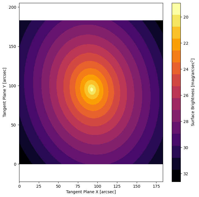
# Plot model image with discrete levels

# this is very useful for visualizing subtle features and for eyeballing the brightness at a given location.
# just add the "cmap_levels" keyword to the model_image call and tell it how many levels you want
fig11, ax11 = plt.subplots(figsize=(8, 8))
ap.plots.model_image(fig11, ax11, model2, cmap_levels=15)
plt.show()

# Save and load a target image

target.save("target.fits")

# Note that it is often also possible to load from regular FITS files
new_target = ap.TargetImage(filename="target.fits")

fig, ax = plt.subplots(figsize=(8, 8))
ap.plots.target_image(fig, ax, new_target)
plt.show()

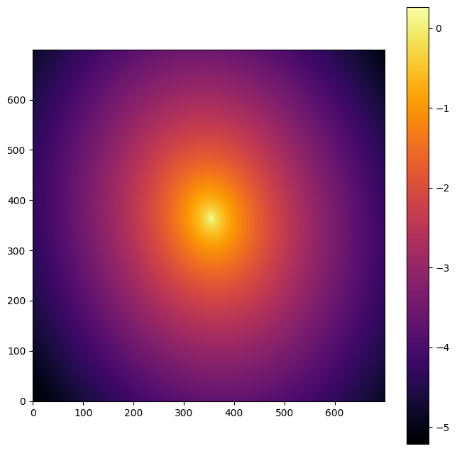
# Access the model image pixels directly

fig2, ax2 = plt.subplots(figsize=(8, 8))

pixels = model2().data.detach().cpu().numpy()

im = plt.imshow(
    np.log10(pixels),  # take log10 for better dynamic range
    origin="lower",
    cmap=ap.plots.visuals.cmap_grad,  # gradient colourmap default for AstroPhot
)
plt.colorbar(im)
plt.show()

Load target with WCS information

# filename = "https://www.legacysurvey.org/viewer/fits-cutout?ra=36.3684&dec=-25.6389&size=700&layer=ls-dr9&pixscale=0.262&bands=r"
# hdu = fits.open(filename)
hdu = fits.open("target_image.fits")
target_data = np.array(hdu[0].data, dtype=np.float64)

wcs = WCS(hdu[0].header)

# Create a target object with WCS which will specify the pixelscale and origin for us!
target = ap.TargetImage(
    data=target_data,
    zeropoint=22.5,
    wcs=wcs,
)

fig3, ax3 = plt.subplots(figsize=(8, 8))
ap.plots.target_image(fig3, ax3, target)
plt.show()

Even better, just load directly from a FITS file

AstroPhot recognizes standard FITS keywords to extract a target image. Note that this wont work for all FITS files, just ones that define the following keywords: CTYPE1, CTYPE2, CRVAL1, CRVAL2, CRPIX1, CRPIX2, CD1_1, CD1_2, CD2_1, CD2_2, and MAGZP with the usual meanings. AstroPhot can also handle SIP, see the SIP tutorial for details there.

Further keywords specific to AstroPhot that it uses for some advanced features like multi-band fitting are: CRTAN1, CRTAN2 used for aligning images, and IDNTY used for identifying when two images are actually cutouts of the same image. And AstroPhot also will store the PSF, WEIGHT, and MASK in extra extensions of the FITS file when it makes one.

target = ap.TargetImage(filename="target_image.fits")

fig3, ax3 = plt.subplots(figsize=(8, 8))
ap.plots.target_image(fig3, ax3, target)
plt.show()

# List all the available model names

# AstroPhot keeps track of all the subclasses of the AstroPhot Model object, this list will
# include all models even ones added by the user
print(ap.Model.List_Models(usable=True, types=True))
print("---------------------------")
# It is also possible to get all sub models of a specific Type
print("only galaxy models: ", ap.models.GalaxyModel.List_Models(types=True))

{'truncated nuker superellipse galaxy model', 'nuker galaxy model', 'ferrer ray galaxy model', 'gaussian galaxy model', 'ferrer psf model', 'gaussianellipsoid model', 'pixelated psf model', 'moffat warp psf model', 'pixelated model', 'truncated ferrer galaxy model', 'truncated gaussian warp galaxy model', 'gaussian wedge galaxy model', 'truncated sersic galaxy model', 'truncated spline superellipse galaxy model', 'moffat superellipse psf model', 'nuker fourier galaxy model', 'spline superellipse galaxy model', 'truncated ferrer warp galaxy model', 'spline superellipse psf model', 'truncated king galaxy model', 'exponential fourier galaxy model', 'exponential superellipse galaxy model', 'spline warp psf model', 'king fourier galaxy model', 'truncated king fourier galaxy model', 'basis psf model', 'batch model', 'spline galaxy model', 'truncated exponential superellipse galaxy model', 'gaussian fourier psf model', 'nuker psf model', 'king galaxy model', 'exponential galaxy model', 'truncated exponential warp galaxy model', 'point model', 'spline ellipse psf model', 'moffat superellipse galaxy model', 'spline warp galaxy model', 'truncated sersic superellipse galaxy model', 'truncated king warp galaxy model', 'truncated sersic warp galaxy model', 'flat sky model', 'ferrer ellipse psf model', 'sersic fourier galaxy model', 'spline psf model', 'truncated ferrer fourier galaxy model', 'sersic ellipse psf model', 'moffat galaxy model', 'spline ray galaxy model', 'spline fourier psf model', 'isothermal sech2 edgeon model', 'sersic superellipse galaxy model', 'truncated nuker fourier galaxy model', 'truncated sersic fourier galaxy model', 'sersic ray galaxy model', 'truncated gaussian galaxy model', 'batch scene model', 'sersic wedge galaxy model', 'moffat warp galaxy model', 'ferrer wedge galaxy model', 'spline fourier galaxy model', 'nuker wedge galaxy model', 'truncated moffat fourier galaxy model', 'ferrer warp psf model', 'moffat ellipse psf model', 'ferrer fourier psf model', 'exponential wedge galaxy model', 'exponential psf model', 'king ellipse psf model', 'sersic superellipse psf model', 'mge model', 'gaussian psf model', 'truncated moffat superellipse galaxy model', 'sersic psf model', 'nuker warp galaxy model', 'truncated spline fourier galaxy model', 'airy psf model', 'truncated exponential galaxy model', 'truncated nuker galaxy model', 'basis model', 'king warp galaxy model', 'king wedge galaxy model', 'ferrer superellipse psf model', 'bilinear sky model', 'gaussian warp galaxy model', 'sersic fourier psf model', 'ferrer superellipse galaxy model', 'truncated nuker warp galaxy model', 'king superellipse galaxy model', 'exponential ellipse psf model', 'gaussian fourier galaxy model', 'nuker superellipse galaxy model', 'ferrer warp galaxy model', 'truncated spline warp galaxy model', 'truncated ferrer superellipse galaxy model', 'exponential fourier psf model', 'sersic warp psf model', 'moffat fourier galaxy model', 'moffat wedge galaxy model', 'truncated gaussian superellipse galaxy model', 'group model', 'nuker superellipse psf model', 'truncated gaussian fourier galaxy model', 'moffat ray galaxy model', 'exponential warp psf model', 'exponential ray galaxy model', 'moffat fourier psf model', 'ferrer fourier galaxy model', 'exponential warp galaxy model', 'king ray galaxy model', 'truncated king superellipse galaxy model', 'king psf model', 'truncated moffat galaxy model', 'nuker ellipse psf model', 'nuker warp psf model', 'ferrer galaxy model', 'truncated spline galaxy model', 'sersic warp galaxy model', 'gaussian ray galaxy model', 'nuker ray galaxy model', 'plane sky model', 'exponential superellipse psf model', 'truncated moffat warp galaxy model', 'sersic galaxy model', 'gaussian superellipse galaxy model', 'king warp psf model', 'gaussian ellipse psf model', 'king superellipse psf model', 'moffat psf model', 'king fourier psf model', 'gaussian superellipse psf model', 'nuker fourier psf model', 'psf group model', 'spline wedge galaxy model', 'truncated exponential fourier galaxy model', 'gaussian warp psf model'}
---------------------------
only galaxy models:  {'truncated nuker superellipse galaxy model', 'nuker galaxy model', 'ferrer ray galaxy model', 'gaussian galaxy model', 'truncated ferrer galaxy model', 'truncated gaussian warp galaxy model', 'gaussian wedge galaxy model', 'truncated sersic galaxy model', 'truncated spline superellipse galaxy model', 'nuker fourier galaxy model', 'spline superellipse galaxy model', 'truncated ferrer warp galaxy model', 'truncated king galaxy model', 'exponential fourier galaxy model', 'exponential superellipse galaxy model', 'king fourier galaxy model', 'truncated king fourier galaxy model', 'spline galaxy model', 'truncated exponential superellipse galaxy model', 'king galaxy model', 'exponential galaxy model', 'truncated exponential warp galaxy model', 'moffat superellipse galaxy model', 'spline warp galaxy model', 'truncated sersic superellipse galaxy model', 'truncated king warp galaxy model', 'truncated sersic warp galaxy model', 'sersic fourier galaxy model', 'truncated ferrer fourier galaxy model', 'moffat galaxy model', 'spline ray galaxy model', 'sersic superellipse galaxy model', 'truncated nuker fourier galaxy model', 'truncated sersic fourier galaxy model', 'sersic ray galaxy model', 'truncated gaussian galaxy model', 'sersic wedge galaxy model', 'moffat warp galaxy model', 'ferrer wedge galaxy model', 'spline fourier galaxy model', 'nuker wedge galaxy model', 'truncated moffat fourier galaxy model', 'exponential wedge galaxy model', 'truncated moffat superellipse galaxy model', 'nuker warp galaxy model', 'truncated spline fourier galaxy model', 'truncated exponential galaxy model', 'truncated nuker galaxy model', 'king warp galaxy model', 'king wedge galaxy model', 'gaussian warp galaxy model', 'ferrer superellipse galaxy model', 'truncated nuker warp galaxy model', 'king superellipse galaxy model', 'gaussian fourier galaxy model', 'nuker superellipse galaxy model', 'ferrer warp galaxy model', 'truncated spline warp galaxy model', 'truncated ferrer superellipse galaxy model', 'moffat fourier galaxy model', 'moffat wedge galaxy model', 'truncated gaussian superellipse galaxy model', 'truncated gaussian fourier galaxy model', 'moffat ray galaxy model', 'exponential ray galaxy model', 'ferrer fourier galaxy model', 'exponential warp galaxy model', 'king ray galaxy model', 'truncated king superellipse galaxy model', 'truncated moffat galaxy model', 'ferrer galaxy model', 'truncated spline galaxy model', 'sersic warp galaxy model', 'gaussian ray galaxy model', 'nuker ray galaxy model', 'truncated moffat warp galaxy model', 'sersic galaxy model', 'gaussian superellipse galaxy model', 'spline wedge galaxy model', 'truncated exponential fourier galaxy model'}

Using GPU acceleration

This one is easy! If you have a cuda enabled GPU available, AstroPhot will just automatically detect it and use that device.

# check if AstroPhot has detected your GPU
print(ap.config.DEVICE)  # most likely this will say "cpu" unless you already have a cuda GPU,
# in which case it should say "cuda:0"

cpu

# If you have a GPU but want to use the cpu for some reason, just set:
ap.config.DEVICE = "cpu"
# BEFORE creating anything else (models, images, etc.)

Boost GPU acceleration with single precision float32

If you are using a GPU you can get significant performance increases in both memory and speed by switching from double precision (the AstroPhot default) to single precision floating point numbers. The trade off is reduced precision, this can cause some unexpected behaviors. For example an optimizer may keep iterating forever if it is trying to optimize down to a precision below what the float32 will track. Typically, numbers with float32 are good down to 6 places and AstroPhot by default only attempts to minimize the Chi^2 to 3 places. However, to ensure the fit is secure to 3 places it often checks what is happenening down at 4 or 5 places. Hence, issues can arise. For the most part you can go ahead with float32 and if you run into a weird bug, try on float64 before looking further.

# Again do this BEFORE creating anything else
ap.config.DTYPE = torch.float32

# Now new AstroPhot objects will be made with single bit precision
T1 = ap.TargetImage(data=np.zeros((100, 100)))
T1.to()
print("now a single:", T1.data.dtype)

# Here we switch back to double precision
ap.config.DTYPE = torch.float64
T2 = ap.TargetImage(data=np.zeros((100, 100)))
T2.to()
print("back to double:", T2.data.dtype)
print("old image is still single!:", T1.data.dtype)

now a single: torch.float32
back to double: torch.float64
old image is still single!: torch.float32

See how the window created as a float32 stays that way? That’s really bad to have lying around! Make sure to change the data type before creating anything!

Tracking output

The AstroPhot optimizers, and occasionally the other AstroPhot objects, will provide status updates about themselves which can be very useful for debugging problems or just keeping tabs on progress. There are a number of use cases for AstroPhot, each having different desired output behaviors. To accommodate all users, AstroPhot implements a general logging system. The object ap.config.logger is a logging object which by default writes to AstroPhot.log in the local directory. As the user, you can set that logger to be any logging object you like for arbitrary complexity. Most users will, however, simply want to control the filename, or have it output to screen instead of a file. Below you can see examples of how to do that.

# note that the log file will be where these tutorial notebooks are in your filesystem

# Here we change the settings so AstroPhot only prints to a log file
ap.config.set_logging_output(stdout=False, filename="AstroPhot.log")
ap.config.logger.info("message 1: this should only appear in the AstroPhot log file")

# Here we change the settings so AstroPhot only prints to console
ap.config.set_logging_output(stdout=True, filename=None)
ap.config.logger.info("message 2: this should only print to the console")

# Here we change the settings so AstroPhot prints to both, which is the default
ap.config.set_logging_output(stdout=True, filename="AstroPhot.log")
ap.config.logger.info("message 3: this should appear in both the console and the log file")

message 2: this should only print to the console

message 3: this should appear in both the console and the log file

You can also change the logging level and/or formatter for the stdout and filename options (see help(ap.config.set_logging_output) for details). However, at that point you may want to simply make your own logger object and assign it to the ap.config.logger variable.