Poisson Noise Model

For the most part, astronomical images are modelled assuming an independent Gaussian uncertainty on every pixel resulting in a negative log likelihood of the form: \(\sum_i\frac{(d_i-m_i)^2}{2\sigma_i^2}\) where \(d_i\) is the pixel value, \(m_i\) is the model value for that pixel, and \(\sigma_i\) is the uncertainty on that pixel. However, in truth the best model for an astronomical image is the Poisson distribution with negative log likelihood of: \(\sum_i m_i + \log(d_i!) - d_i\log(m_i)\) with the same definitions, except specifying that \(d_i\) is in counts (number of photons or electrons). For large enough \(d_i\) these likelihoods are essentially identical and Gaussian is easier to work with. When signal-to-noise ratios get very low, the differences between Poisson and Gaussian distributions can become apparent and so it is important to treat the data with a Poisson likelihood. These conditions regularly occur for gamma ray, x-ray, and low SNR UV data, but are less common for longer wavelengths. AstroPhot can model Poisson likelihood data, here we will demo an example.

import astrophot as ap
import numpy as np
import matplotlib.pyplot as plt

Make some mock data

Lets create some mock low SNR data. Notice that poisson noise isn’t additive like gaussian noise. To sample the image, out true model acts as a photon rate and the np.random.poisson samples some number of counts based on that rate. Our goal will be to recover the rate of every pixel and ultimately the sersic parameters that produce the correct rate model.

# make some mock data
target = ap.TargetImage(data=np.zeros((128, 128)))
true_model = ap.Model(
    name="truth",
    model_type="sersic galaxy model",
    center=(64, 64),
    q=0.7,
    PA=0.5,
    n=1,
    Re=32,
    Ie=1,
    target=target,
)
img = true_model().data.detach().cpu().numpy()
np.random.seed(42)  # for reproducibility
target.data = np.random.poisson(img)  # sample poisson distribution
true_params = true_model.get_values()

fig, ax = plt.subplots(1, 2, figsize=(10, 5))
ap.plots.model_image(fig, ax[0], true_model)
ax[0].set_title("True Model")
ap.plots.target_image(fig, ax[1], target)
ax[1].set_title("Target Image (Poisson Sampled)")
plt.show()

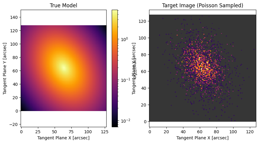
Indeed this is some noisy data. The AstroPhot target_image plotting routine struggles a bit with this image, but it kind of looks neat anyway.

Model the data

model = ap.Model(name="model", model_type="sersic galaxy model", target=target)
model.initialize()

While the Levenberg-Marquardt algorithm is traditionally considered as a least squares algorithm, that is actually just its most common application. LM naturally generalizes to a broad class of problems, including the Poisson Likelihood (see Fowler 2014). Here we see the AstroPhot automatic initialization does well on this image and recovers decent starting parameters, LM has an easy time finishing the job to find the maximum likelihood.

Note that the idea of a \(\chi^2/{\rm dof}\) is not as clearly defined for a Poisson likelihood. We take the closest analogue by taking 2 times the negative log likelihood divided by the DoF. This doesn’t have any strict statistical meaning but is somewhat intuitive to work with for those used to \(\chi^2/{\rm dof}\).

res = ap.fit.LM(model, likelihood="poisson", verbose=1).fit()

fig, ax = plt.subplots()
ap.plots.model_image(fig, ax, model)
ax.set_title("Fitted Model")
plt.show()

==Starting LM fit for 'model' with 7 dynamic parameters and 16384 pixels==

2NLL/DoF: 1.13152, L: 1

/home/docs/checkouts/readthedocs.org/user_builds/astrophot/envs/v0.17.3/lib/python3.12/site-packages/torch/jit/_script.py:1488: DeprecationWarning: `torch.jit.script` is deprecated. Please switch to `torch.compile` or `torch.export`.
  warnings.warn(

2NLL/DoF: 1.07502, L: 1

2NLL/DoF: 1.05025, L: 0.000152

2NLL/DoF: 1.04935, L: 2.32e-08

Final 2NLL/DoF: 1.04935, L: 2.32e-08. Converged: success

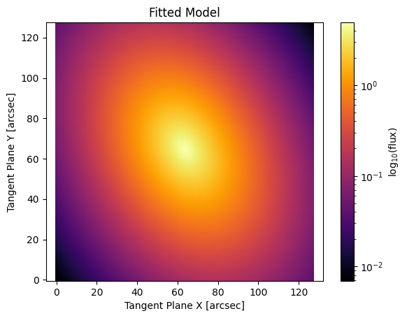
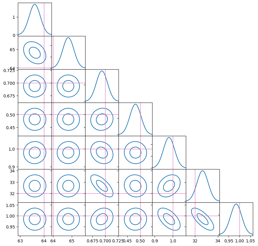
Plotting the model parameters and uncertainty, we see that we have indeed recovered very close to the true values for all parameters! Note that the true values are, however, not where we expect with respect to the 1-2 sigma uncertainty contours. There are two reasons for this, one is that this is a Poisson likelihood and so a Gaussian approximation is only so good, the other is that the model is non-linear so again the Gaussian approximation at the maximum likelihood will not exactly describe the PDF (which actually affects model uncertainties even for a Gaussian likelihood).

fig, ax = ap.plots.covariance_matrix(
    res.covariance_matrix.detach().cpu().numpy(),
    model.get_values().detach().cpu().numpy(),
    reference_values=true_params.detach().cpu().numpy(),
)
plt.show()

If you encounter a problem where LM struggles to fit the poisson data, the Slalom optimizer is also quite efficient in these settings. See the fitting methods tutorial for more details.