Fitting with Priors

AstroPhot is mostly built around likelihood optimization under the assumption that the prior is encoded in the allows model parameter space. However, this is not always enough, sometimes we need to more explicitly provide a prior. The most general way to add a prior is to entirely code it up yourself. Every AstroPhot model gives you access to model.gaussian_log_likelihood and model.poisson_log_likelihood functions which take as input a vector of parameter values (which you can get for any given model by calling model.get_values()). Thus you may create a prior function which takes the same vector of parameters as input and off you go for a fully Bayesian analysis.

But there is a middle ground. The LM fitter includes the ability to add a Gaussian prior on your model parameters (this only works for the Gaussian likelihood!). It does this by essentially adding fake “zero flux pixels” to the fit where the value in those pixels from the model is up to you. So you can have those “pixels” take values from your model parameters and thus you have a prior! The actual system is more general and allows for quite complex constraints on your parameters (for example you could preferentially have one radius larger than another).

%matplotlib inline
%load_ext autoreload
%autoreload 2

import astrophot as ap
import numpy as np
import torch
import matplotlib.pyplot as plt

First, lets make some fake data to analyze

target = ap.TargetImage(data=torch.zeros(32, 32))
true_model = ap.Model(
    name="true_model",
    model_type="sersic galaxy model",
    target=target,
    center=[16.0, 16.0],
    q=0.4,
    PA=np.pi / 3,
    n=1,
    Re=4,
    Ie=10,
)

sample = true_model().data
torch.manual_seed(61803398)
target.data = sample + torch.normal(torch.zeros_like(sample), torch.sqrt(1 + sample))
target.variance = 1 + sample

fig, ax = plt.subplots(1, 2, figsize=(16, 7))
ap.plots.model_image(fig, ax[0], true_model)
ap.plots.target_image(fig, ax[1], target)
ax[0].set_title("true sersic model")
ax[1].set_title("mock observed data")
plt.show()

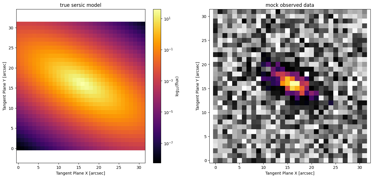
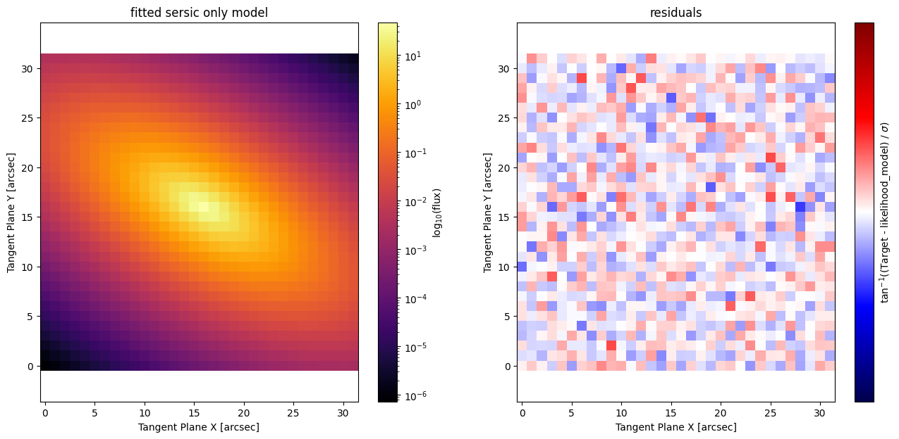
This is some pretty noisy data! lets see what happens when we fit it

likelihood_model = ap.Model(
    name="likelihood_model",
    model_type="sersic galaxy model",
    target=target,
)
likelihood_model.initialize()
print(likelihood_model)
res = ap.fit.LM(likelihood_model).fit()

fig, ax = plt.subplots(1, 2, figsize=(16, 7))
ap.plots.model_image(fig, ax[0], likelihood_model)
ap.plots.residual_image(fig, ax[1], likelihood_model, normalize_residuals=True)
ax[0].set_title("fitted sersic only model")
ax[1].set_title("residuals")
plt.show()
print(likelihood_model)

likelihood_model|SersicGalaxy
    TargetImage|TargetImage
        crtan|static: [0, 0]
        crval|static: [0, 0]
        CD|static: [[1, 0], [0, 1]]
    center|dynamic: [15.8, 16.2]
    q|dynamic: 0.257
    PA|dynamic: 0.885
    n|dynamic: 3.21
    Re|dynamic: 11.7
    Ie|dynamic: 1.78
==Starting LM fit for 'likelihood_model' with 7 dynamic parameters and 1024 pixels==

Chi^2/DoF: 1.19224, L: 1

/home/docs/checkouts/readthedocs.org/user_builds/astrophot/envs/v0.17.3/lib/python3.12/site-packages/torch/jit/_script.py:1488: DeprecationWarning: `torch.jit.script` is deprecated. Please switch to `torch.compile` or `torch.export`.
  warnings.warn(

Chi^2/DoF: 1.05658, L: 0.0123

Chi^2/DoF: 0.989049, L: 0.0123

Chi^2/DoF: 0.967482, L: 0.0123

Chi^2/DoF: 0.96659, L: 2.32e-08

Chi^2/DoF: 0.966576, L: 2.32e-08

Final Chi^2/DoF: 0.966576, L: 2.32e-08. Converged: success

likelihood_model|SersicGalaxy
    TargetImage|TargetImage
        crtan|static: [0, 0]
        crval|static: [0, 0]
        CD|static: [[1, 0], [0, 1]]
    center|dynamic: [15.9, 16]
    q|dynamic: 0.444
    PA|dynamic: 1.04
    n|dynamic: 1.17
    Re|dynamic: 3.73
    Ie|dynamic: 9.73

posterior_model = ap.Model(
    name="posterior_model",
    model_type="sersic galaxy model",
    target=target,
    n=1,
)
posterior_model.initialize()

# This is the constraint, the first argument is the model to constrain, the
# second is a function (that takes the model as an argument) for which values
# closer to zero are better, and the third argument is the sigma of the gaussian
# constraint/prior. The sigma and the function output need to be a vector (even
# if its only one element like in this case).
C = ap.fit.LMConstraint(posterior_model, lambda m: m.n.value[None] - 1.0, np.array([1e-1]))

res = ap.fit.LM(posterior_model, constraint=C).fit()

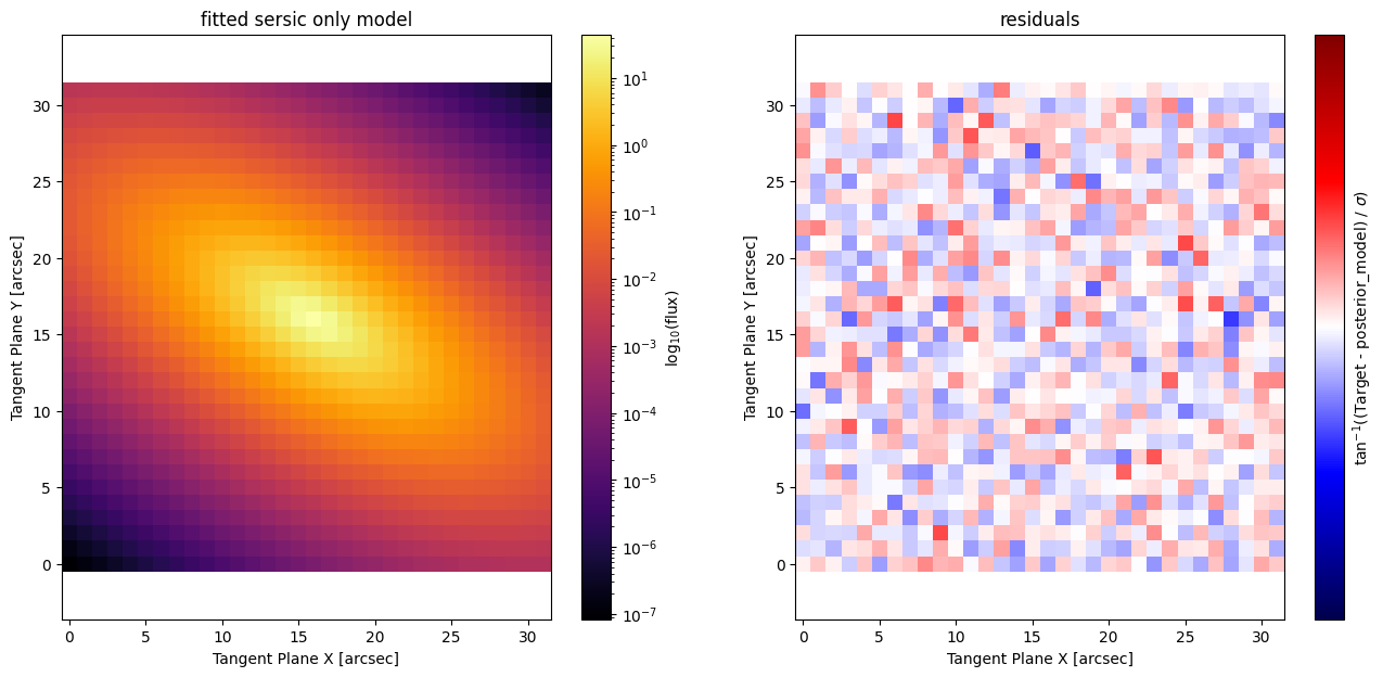
fig, ax = plt.subplots(1, 2, figsize=(16, 7))
ap.plots.model_image(fig, ax[0], posterior_model)
ap.plots.residual_image(fig, ax[1], posterior_model, normalize_residuals=True)
ax[0].set_title("fitted sersic only model")
ax[1].set_title("residuals")
plt.show()
print(posterior_model)

==Starting LM fit for 'posterior_model' with 7 dynamic parameters and 1025 pixels==

Chi^2/DoF: 1.20124, L: 1

Chi^2/DoF: 1.01953, L: 0.0123

Chi^2/DoF: 0.967383, L: 0.0123

Chi^2/DoF: 0.966793, L: 2.32e-08

Final Chi^2/DoF: 0.966791, L: 2.32e-08. Converged: success

posterior_model|SersicGalaxy
    TargetImage|TargetImage
        crtan|static: [0, 0]
        crval|static: [0, 0]
        CD|static: [[1, 0], [0, 1]]
    center|dynamic: [15.9, 16]
    q|dynamic: 0.444
    PA|dynamic: 1.04
    n|dynamic: 1.07
    Re|dynamic: 3.7
    Ie|dynamic: 10.2

Here we see the prior has pushed our sersic index closer to an exponential disk, without strictly enforcing a value of 1.

Note: Once you add a prior, the LM fitter update messages that say “Chi^2/DoF: …” are actually now more appropriately called “two times the log posterior density divided by the number of degrees of freedom”, which is a bit of a mouthful. For the most part you don’t need to worry too much, a value near 1 is still good. You can contact me if you have more detailed questions.

Soft equality constraints

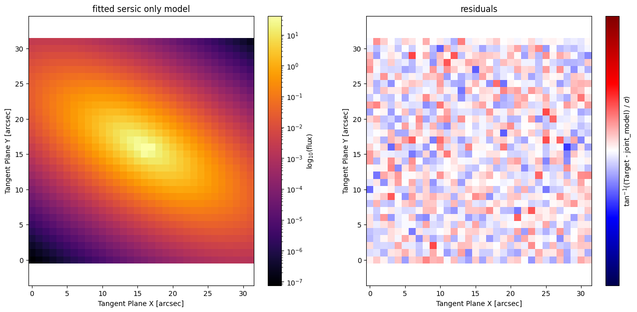
There are tons of applications for these priors/constraints, another one we will consider here is the idea of a two component model, that has a soft constraint that the centers of the two models align. Lets just fit the same data and see what happens!

model1 = ap.Model(
    name="model1",
    model_type="sersic galaxy model",
    target=target,
    n=1,
    Re=3,
)
model2 = ap.Model(
    name="model2",
    model_type="sersic galaxy model",
    target=target,
    n=2,
    Re=5,
)
joint_model = ap.Model(
    name="joint_model",
    model_type="group model",
    target=target,
    models=[model1, model2],
)
joint_model.initialize()

# Constrain both models to have roughly the same position and to have n near 1.0
C = ap.fit.LMConstraint(
    joint_model,
    lambda m: torch.concatenate(
        [
            m.models.model1.center.value - m.models.model2.center.value,
            m.models.model1.n.value[None] - 1.0,
            m.models.model2.n.value[None] - 1.0,
        ]
    ),
    np.array([1.0, 1.0, 1e-1, 1e-1]),
)

res = ap.fit.LM(joint_model, constraint=C).fit()

fig, ax = plt.subplots(1, 2, figsize=(16, 7))
ap.plots.model_image(fig, ax[0], joint_model)
ap.plots.residual_image(fig, ax[1], joint_model, normalize_residuals=True)
ax[0].set_title("fitted sersic only model")
ax[1].set_title("residuals")
plt.show()
print(joint_model)

Initializing model model1

Initializing model model2

==Starting LM fit for 'joint_model' with 14 dynamic parameters and 1028 pixels==

Chi^2/DoF: 1.17993, L: 1

Chi^2/DoF: 1.03882, L: 1

Chi^2/DoF: 0.974584, L: 0.0123

Chi^2/DoF: 0.968022, L: 0.00137

Chi^2/DoF: 0.964186, L: 0.00137

Chi^2/DoF: 0.961941, L: 0.00137

Chi^2/DoF: 0.960455, L: 0.000152

Chi^2/DoF: 0.959172, L: 2.32e-08

Chi^2/DoF: 0.959015, L: 0.00374

Chi^2/DoF: 0.958904, L: 0.0412

Chi^2/DoF: 0.958676, L: 0.0412

Chi^2/DoF: 0.958647, L: 0.453

Chi^2/DoF: 0.958541, L: 0.00559

Chi^2/DoF: 0.958503, L: 1.05e-08

Chi^2/DoF: 0.9585, L: 0.205

Chi^2/DoF: 0.958495, L: 2.25

Chi^2/DoF: 0.958463, L: 5.24e-08

Chi^2/DoF: 0.958447, L: 5.24e-08

Chi^2/DoF: 0.958444, L: 1.02

Chi^2/DoF: 0.958434, L: 2.37e-08

Final Chi^2/DoF: 0.958432, L: 2.37e-08. Converged: success

joint_model|GroupModel
    TargetImage|TargetImage
        crtan|static: [0, 0]
        crval|static: [0, 0]
        CD|static: [[1, 0], [0, 1]]
    models|nlist
        model1|SersicGalaxy
            TargetImage|TargetImage
                crtan|static: [0, 0]
                crval|static: [0, 0]
                CD|static: [[1, 0], [0, 1]]
            center|dynamic: [16.6, 15.6]
            q|dynamic: 0.22
            PA|dynamic: 2.22
            n|dynamic: 0.999
            Re|dynamic: 0.857
            Ie|dynamic: 22.5
        model2|SersicGalaxy
            TargetImage|TargetImage
                crtan|static: [0, 0]
                crval|static: [0, 0]
                CD|static: [[1, 0], [0, 1]]
            center|dynamic: [15.8, 16.1]
            q|dynamic: 0.435
            PA|dynamic: 1.03
            n|dynamic: 1.04
            Re|dynamic: 3.95
            Ie|dynamic: 8.76

Success! Notice how the two models have a similar, but not identical position.

This is a very powerful method to stabilize fitting and avoid bad areas of parameter space. Just keep in mind that adding more constraints can make it difficult for the fitter to find the optimal parameter values. Sometimes a constraint will block off a path through parameter space and so things can get stuck. It’s best not to assume anything when the number of parameters gets large since high dimensional spaces can be confusing.